From target to projectile: CSS evolution of quark TMD in different light-cone gauges
Pith reviewed 2026-06-26 23:54 UTC · model grok-4.3
The pith
The CSS evolution equations for the quark TMD are recovered after its one-loop renormalization in the projectile light-cone gauge.
A machine-rendered reading of the paper's core claim, the machinery that carries it, and where it could break.
Core claim
After one-loop renormalization of the quark TMD in the projectile light-cone gauge using the Mandelstam-Leibbrandt prescription and the pure rapidity regulator, the Collins-Soper-Sterman evolution equations are recovered and the rapidity divergences exhibit the same structure found in the target light-cone gauge.
What carries the argument
One-loop renormalization of the quark TMD in the projectile light-cone gauge with the Mandelstam-Leibbrandt prescription and pure rapidity regulator, which produces the CSS kernel.
If this is right
- The CSS evolution kernel is the same in the projectile and target light-cone gauges.
- Double-logarithmic contributions to the resummation remain consistent across the two gauges.
- The result supports equivalence between TMD factorization and the Color Glass Condensate description at this order.
Where Pith is reading between the lines
- Gauge choice between target and projectile frames can be made for computational convenience without changing the extracted evolution kernel.
- The same regularization approach may be tested on gluon TMDs or other distributions.
- Numerical implementations of TMD evolution could adopt either gauge depending on the kinematic setup.
Load-bearing premise
The Mandelstam-Leibbrandt prescription combined with the pure rapidity regulator captures all rapidity divergences at one loop without introducing artifacts that alter the CSS kernel.
What would settle it
A mismatch between the CSS kernel extracted at two loops in the projectile gauge and the kernel already known from the target gauge.
Figures
read the original abstract
We calculate the one-loop corrections to the quark TMD in the projectile light-cone gauge using the background field formalism, with the Mandelstam-Leibbrandt (ML) prescription for the extra singularity present in the light-cone gauge propagator. We use the pure rapidity regulator for rapidity divergences. The Collins-Soper-Sterman (CSS) evolution equations are obtained after one-loop renormalization of the quark TMD in this gauge. We discuss how the structure of the rapidity divergences and the double-logarithmic contributions to the CSS resummation compares with the analogous calculation performed in the target light-cone gauge, and discuss the implications for the connection between the TMD factorization and Color Glass Condensate frameworks.
Editorial analysis
A structured set of objections, weighed in public.
Referee Report
Summary. The manuscript computes the one-loop corrections to the quark TMD in the projectile light-cone gauge within the background-field formalism, employing the Mandelstam-Leibbrandt prescription for the gauge propagator and a pure rapidity regulator. After renormalization it recovers the standard Collins-Soper-Sterman evolution equations and compares the structure of rapidity divergences together with the double-logarithmic contributions to the corresponding calculation performed in the target light-cone gauge, with remarks on the interface between TMD factorization and the Color Glass Condensate framework.
Significance. If the regulator combination is shown to reproduce the universal rapidity anomalous dimension without artifacts, the result supplies a direct gauge-independence check of the CSS kernel between target and projectile light-cone gauges. This would strengthen the theoretical link between TMD resummation and high-energy effective theories and provide a concrete test of factorization assumptions that are otherwise taken from covariant-gauge calculations.
major comments (1)
- [calculation of the rapidity anomalous dimension (one-loop diagrams and renormalization)] The central claim that the ML prescription plus pure rapidity regulator yields exactly the standard CSS kernel rests on the absence of spurious rapidity-divergent or finite terms. The manuscript must therefore exhibit the explicit one-loop rapidity anomalous dimension (or the coefficient of the double logarithm) and demonstrate its numerical and analytic agreement with the known result from covariant or target-gauge calculations; any residual scheme-dependent piece would render the extracted kernel non-universal.
minor comments (2)
- Notation for the light-cone vectors and the precise definition of the pure rapidity regulator should be stated once at the beginning of the technical section to avoid ambiguity when comparing with the target-gauge literature.
- The abstract states that the structures are compared, but the manuscript would benefit from a compact table or side-by-side list of the divergent and finite pieces obtained in each gauge.
Simulated Author's Rebuttal
We thank the referee for the careful reading and the constructive major comment. We respond point by point below.
read point-by-point responses
-
Referee: [calculation of the rapidity anomalous dimension (one-loop diagrams and renormalization)] The central claim that the ML prescription plus pure rapidity regulator yields exactly the standard CSS kernel rests on the absence of spurious rapidity-divergent or finite terms. The manuscript must therefore exhibit the explicit one-loop rapidity anomalous dimension (or the coefficient of the double logarithm) and demonstrate its numerical and analytic agreement with the known result from covariant or target-gauge calculations; any residual scheme-dependent piece would render the extracted kernel non-universal.
Authors: We agree that explicit exhibition of the one-loop rapidity anomalous dimension is required to confirm the absence of spurious terms. Our calculation of the one-loop diagrams in the projectile light-cone gauge with the ML prescription and pure rapidity regulator yields, after renormalization, the standard CSS evolution equations. The structure of the rapidity divergences and the coefficient of the double logarithm are shown to match those obtained in the target light-cone gauge (and, by extension, covariant-gauge results), with no residual scheme-dependent pieces. To make this fully transparent as requested, we will add an explicit statement of the one-loop rapidity anomalous dimension (including its numerical value) together with an analytic comparison to the known literature result in the revised manuscript. revision: yes
Circularity Check
Direct perturbative one-loop renormalization derives CSS equations independently
full rationale
The paper executes an explicit one-loop calculation of quark TMD corrections in the projectile light-cone gauge via background field formalism, Mandelstam-Leibbrandt prescription, and pure rapidity regulator. CSS evolution equations emerge directly from renormalization of the computed TMD. No equation or result reduces by construction to a fitted input, self-defined quantity, or load-bearing self-citation; comparisons to target-gauge results function as external validation rather than foundational premises. The derivation chain is self-contained against the stated perturbative inputs and regulators.
Axiom & Free-Parameter Ledger
Reference graph
Works this paper leans on
-
[1]
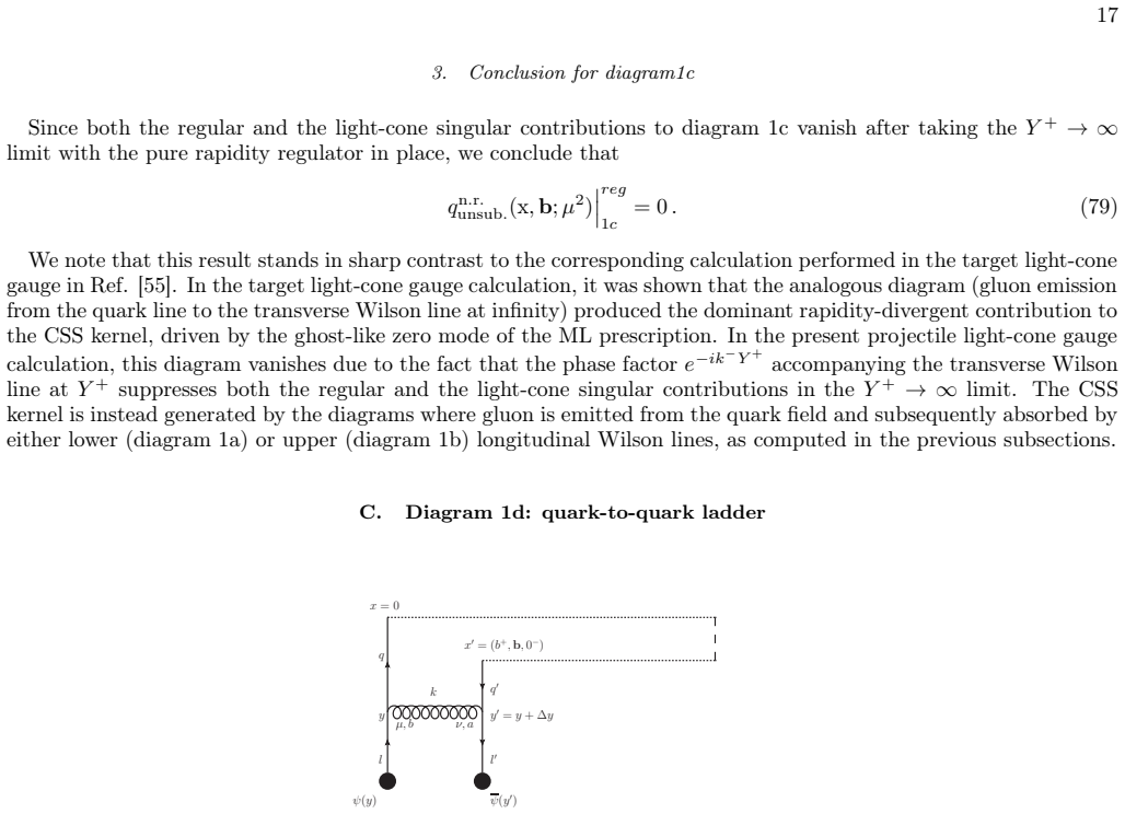
After the spacetime translation (10), its contribution reads qn.r
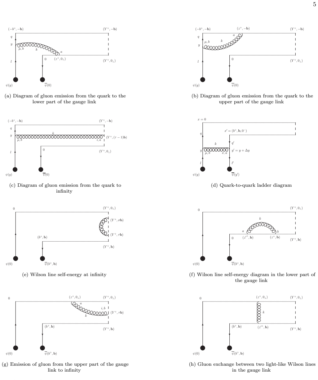
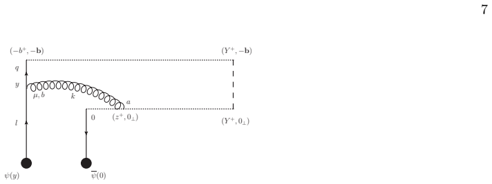
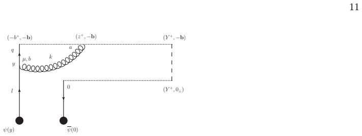
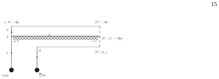
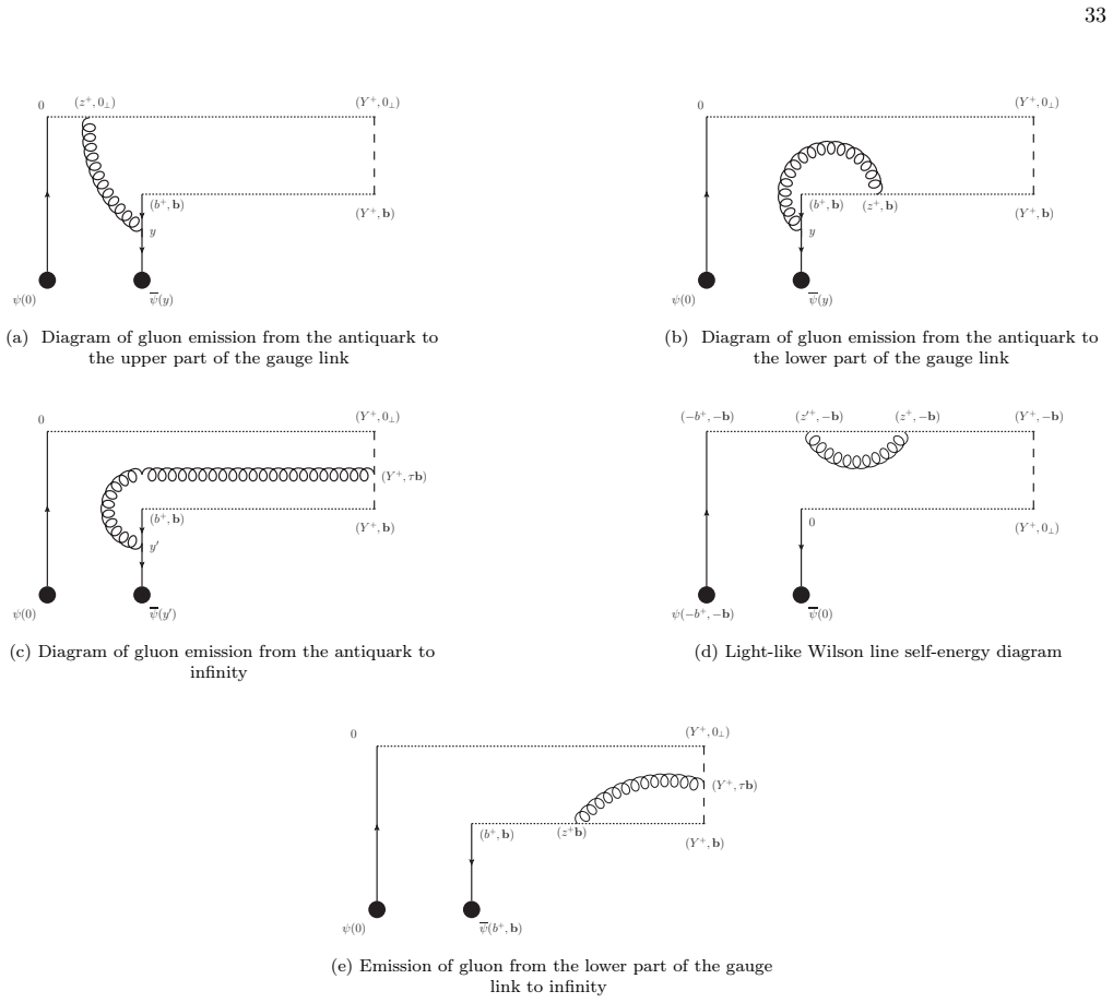
Diagram 1b Diagram1bcorrespondstoradiationofagluonfromthequarkfieldwhichisthenabsorbedbytheupperlongitudinal Wilson line of the staple. After the spacetime translation (10), its contribution reads qn.r. unsub.(x,b;µ 2) 1b = lim Y +→+∞ Z db+ (2π) e−ixP −b+ × P T h ψ(0) γ− 2 ( −iµϵg Z Y + −b+ dz+taδA− a (z+,−b,0 −) ) δΨ(−b+,−b,0 −) i P c .(44) Expressing th...
-
[2]
(38) and (58), respectively
Combined rapidity-divergent contribution from Diagram 1a and Diagram 1b The rapidity-divergent parts of diagram 1a and diagram 1b are given in Eqs. (38) and (58), respectively. Combining these two expressions, we obtain qn.r. unsub.(x,b;µ 2, ζ) 1/η 1a+1b =− αsµ2ϵCF 2π [xP −]η w2 2ν+ ν− η 2 1 η Z d4−2ϵy P ψ(0)γ − ψ(y) P eixP −y+ × Z d2−2ϵl (2π)2−2ϵ Z dl+ (...
-
[3]
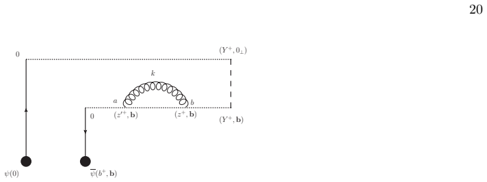
The contribution of theseregularterms to diagram 1c takes the following form qn.r
Regular contribution For the regular terms, thek+ integral takes the form Ireg ≡ Z dk+ 2π 1 2k− k+ − k2−i0 2k− 1 (−2xP −) h k+ −l + + (l−k)2−i0 2xP − i = −iθ(k−) 2 [2xP−k−l+ −xP −k2 −k −(l−k) 2] ,(72) where the contour has been closed below the real axis using the constraintY+ −y + >0, and contributions from negativek − vanish since all poles lie on the s...
-
[4]
(70)), one finds ILC ∼ −ixP − θ(k−) l4 k− −xP − k2 l2 ,(77) wherel 2 = 2xP −l+ −l 2
Contribution with the extra light-cone gauge singularity For the term containing the extra light-cone gauge singularity1/[k+], thek + integral with the ML prescription (26) reads ILC ≡ Z dk+ 2π 1 2k− k+ − k2−i0 2k− 1 (−2xP −) h k+ −l + + (l−k)2−i0 2xP − i ( θ(k−) k+ +i0 + θ(−k−) k+ −i0 ) .(76) Applying contour integration and performing the shiftl→l+k, wh...
-
[5]
unsub.(x,b;µ 2) reg 1c = 0.(79) We note that this result stands in sharp contrast to the corresponding calculation performed in the target light-cone gauge in Ref
Conclusion for diagram1c Since both the regular and the light-cone singular contributions to diagram 1c vanish after taking theY+ → ∞ limit with the pure rapidity regulator in place, we conclude that qn.r. unsub.(x,b;µ 2) reg 1c = 0.(79) We note that this result stands in sharp contrast to the corresponding calculation performed in the target light-cone g...
-
[6]
It arises from the fifth term in the background field expansion (18) and can be written as qn.r
Diagram 1f: Wilson line self-energy on the lower part of the gauge link Diagram 1f corresponds to the one-loop self-energy of the lower longitudinal Wilson line, running from0toY+ at b. It arises from the fifth term in the background field expansion (18) and can be written as qn.r. unsub.(x,b;µ 2) 1f = lim Y +→+∞ Z db+ (2π) e−ixP −b+D P T h ψ(b+,b,0 −) γ−...
-
[7]
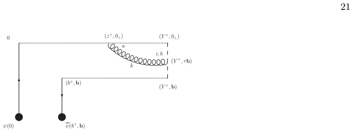
It arises from the seventh term in the background field expansion (18) and can be written as qn.r
Diagram 1g: Gluon emission from the upper part of the gauge link to infinity Diagram 1g corresponds to gluon emission from the lower longitudinal Wilson line at0⊥ to the transverse Wilson line at light-cone infinityY +. It arises from the seventh term in the background field expansion (18) and can be written as qn.r. unsub.(x,b;µ 2) 1g = lim Y +→+∞ Z db+ ...
-
[8]
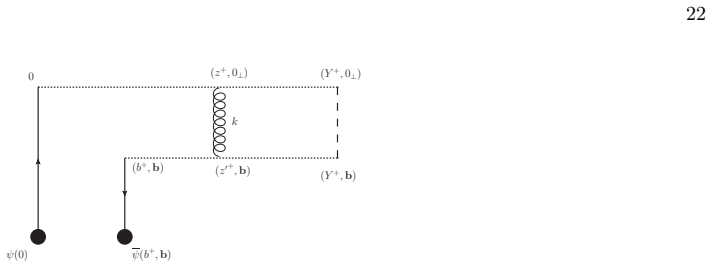
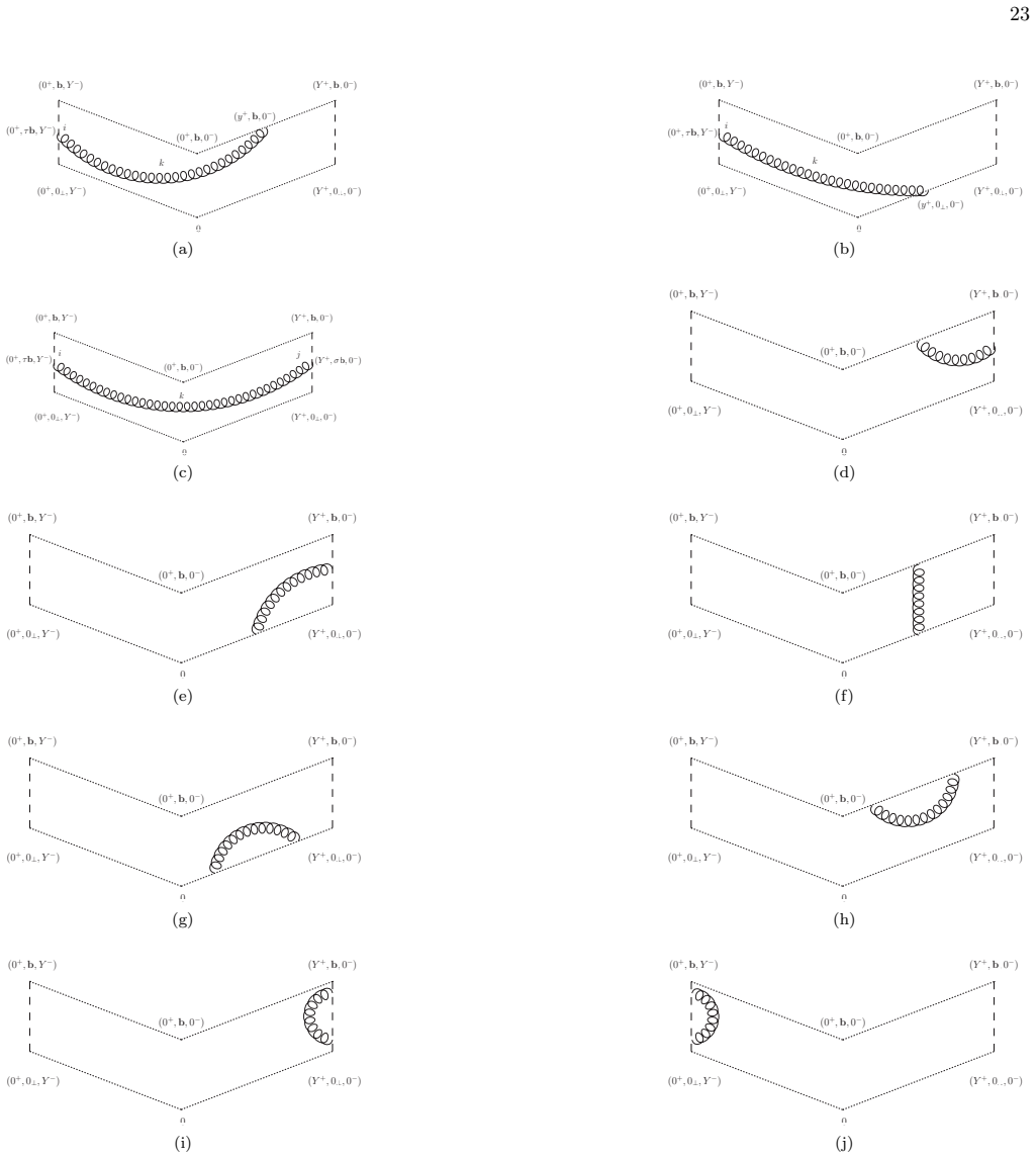
It arises from the eighth term in 22 0 (Y +, 0⊥ ) ψ(0) ψ(b+, b) (Y +, b)(b+, b) k (z+, 0⊥ ) (z′+, b) FIG
Diagram 1h: Gluon exchange between the two longitudinal Wilson lines Diagram 1h corresponds to the exchange of a gluon between the lower longitudinal Wilson line (running fromb+ toY + atb) and the upper longitudinal Wilson line (running from0toY + at0 ⊥). It arises from the eighth term in 22 0 (Y +, 0⊥ ) ψ(0) ψ(b+, b) (Y +, b)(b+, b) k (z+, 0⊥ ) (z′+, b) ...
-
[9]
Summary for diagrams 1f, 1g and 1h All three diagrams 1f, 1g and 1h vanish identically in the projectile light-cone gauge. The vanishing mechanism is the same in each case: the gluon propagator components˜G−− 0,F and ˜Gi− 0,F, which are the only ones that can appear in these diagrams, carry the extra light-cone gauge singularity1/[k+]from the ML prescript...
-
[10]
Diagram 9a The contribution to the soft factor given by the diagram 9a can be written as S(b) 9a =− 1 2 g2µ2ϵCF lim Y ±→+∞ Z d4−2ϵk (2π)4−2ϵ i e−ik+Y − k2 +i0 (−ki) [k+] Z Y + 0 dy+ eik−y+ Z 1 0 dτb i e−iτk·b .(109) After performing the integrations overy+ andτ, one can reorganize the expression as S(b) 9a = 1 2 g2µ2ϵCF lim Y ±→+∞ Z d2−2ϵk (2π)2−2ϵ i e−ik...
-
[11]
Diagram 9b The contribution from diagram 9b differs from that of diagram 9a by an overall sign, which arises from the reversed direction of integration along the upper longitudinal Wilson line, and by an additional phase factoreik·b reflecting the transverse displacement. Specifically, S(b) 9b =− 1 2 g2µ2ϵCF lim Y ±→+∞ Z d4−2ϵk (2π)4−2ϵ ie−ik+Y − k2 +i0 (...
-
[12]
Diagram 9c Diagram 9c involves a gluon connecting the two transverse Wilson lines atY+ andY −, located at transverse positionsτbandσbrespectively. Its contribution reads S(b) 9c =− 1 2 g2µ2ϵCF lim Y ±→+∞ Z d4−2ϵk (2π)4−2ϵ i k2 +i0 Z 1 0 dσb j e−ik−Y ++iσk·b Z 1 0 dτb i eik+Y −−iτk·b .(116) Performing the contour integration overk+ in the same way as for d...
-
[13]
These diagrams involve only the transverse gluon propagator given in Eq
Diagrams 9i and 9j The remaining non-vanishing contributions to the soft factor come from diagrams 9i and 9j which corresponds to the gluon loop on the two space-like Wilson lines at light-cone infinityY+ →+∞andY − →+∞, respectively. These diagrams involve only the transverse gluon propagator given in Eq. (108), and does not carry an extra light-cone gaug...
-
[14]
Rap. div
Total soft factor Combining all contributions, the one-loop soft factor in the projectile light-cone gauge in pure rapidity regularization is S(b) = 1 + αsCF π (πµ2b2)ϵ Γ(1−ϵ) ϵ(1−2ϵ) +O(α 2 s).(121) This result is identical to the soft factor used in the target light-cone gauge calculation of Ref. [55]. Due to the symmetry between the+and−directions in t...
2023
-
[15]
C. J. Bomhof, P. J. Mulders, and F. Pijlman, Eur. Phys. J. C47, 147 (2006), arXiv:hep-ph/0601171
Pith/arXiv arXiv 2006
-
[16]
A. Bacchetta, M. Diehl, K. Goeke, A. Metz, P. J. Mulders, and M. Schlegel, JHEP02, 093 (2007), arXiv:hep-ph/0611265
Pith/arXiv arXiv 2007
-
[17]
Collins,Foundations of Perturbative QCD, Cambridge Monographs on Particle Physics, Nuclear Physics and Cosmology, Vol
J. Collins,Foundations of Perturbative QCD, Cambridge Monographs on Particle Physics, Nuclear Physics and Cosmology, Vol. 32 (Cambridge University Press, 2023)
2023
-
[18]
Angeles-Martinezet al., Acta Phys
R. Angeles-Martinezet al., Acta Phys. Polon. B46, 2501 (2015), arXiv:1507.05267 [hep-ph]
Pith/arXiv arXiv 2015
-
[19]
Boussarieet al., (2023), arXiv:2304.03302 [hep-ph]
R. Boussarieet al., (2023), arXiv:2304.03302 [hep-ph]
arXiv 2023
-
[20]
F. Gelis, E. Iancu, J. Jalilian-Marian, and R. Venugopalan, Ann. Rev. Nucl. Part. Sci.60, 463 (2010), arXiv:1002.0333 [hep-ph]. 36
Pith/arXiv arXiv 2010
-
[21]
J. L. Albacete and C. Marquet, Prog. Part. Nucl. Phys.76, 1 (2014), arXiv:1401.4866 [hep-ph]
Pith/arXiv arXiv 2014
-
[22]
J.-P. Blaizot, Rept. Prog. Phys.80, 032301 (2017), arXiv:1607.04448 [hep-ph]
Pith/arXiv arXiv 2017
-
[23]
J. C. Collins and D. E. Soper, Nucl. Phys. B193, 381 (1981), [Erratum: Nucl.Phys.B 213, 545 (1983)]
1981
-
[24]
J. C. Collins and D. E. Soper, Nucl. Phys. B194, 445 (1982)
1982
-
[25]
J. C. Collins, D. E. Soper, and G. F. Sterman, Nucl. Phys. B250, 199 (1985)
1985
-
[26]
Mandelstam, Nucl
S. Mandelstam, Nucl. Phys. B213, 149 (1983)
1983
-
[27]
Leibbrandt, Phys
G. Leibbrandt, Phys. Rev. D29, 1699 (1984)
1984
-
[28]
Leibbrandt and S.-L
G. Leibbrandt and S.-L. Nyeo, Phys. Lett. B140, 417 (1984)
1984
-
[29]
Bassetto, M
A. Bassetto, M. Dalbosco, I. Lazzizzera, and R. Soldati, Phys. Rev. D31, 2012 (1985)
2012
- [30]
-
[31]
Y. V. Kovchegov, Phys. Rev. D60, 034008 (1999), arXiv:hep-ph/9901281
Pith/arXiv arXiv 1999
-
[32]
Y. V. Kovchegov, Phys. Rev. D61, 074018 (2000), arXiv:hep-ph/9905214
Pith/arXiv arXiv 2000
-
[33]
J. Jalilian-Marian, A. Kovner, L. D. McLerran, and H. Weigert, Phys. Rev. D55, 5414 (1997), arXiv:hep-ph/9606337
Pith/arXiv arXiv 1997
-
[34]
J. Jalilian-Marian, A. Kovner, A. Leonidov, and H. Weigert, Nucl. Phys. B504, 415 (1997), arXiv:hep-ph/9701284
Pith/arXiv arXiv 1997
-
[35]
J. Jalilian-Marian, A. Kovner, A. Leonidov, and H. Weigert, Phys. Rev. D59, 014014 (1998), arXiv:hep-ph/9706377
Pith/arXiv arXiv 1998
-
[36]
J. Jalilian-Marian, A. Kovner, and H. Weigert, Phys. Rev. D59, 014015 (1998), arXiv:hep-ph/9709432
Pith/arXiv arXiv 1998
-
[37]
A. Kovner, J. G. Milhano, and H. Weigert, Phys. Rev. D62, 114005 (2000), arXiv:hep-ph/0004014
Pith/arXiv arXiv 2000
- [38]
-
[39]
E. Iancu, A. Leonidov, and L. D. McLerran, Nucl. Phys. A692, 583 (2001), arXiv:hep-ph/0011241
Pith/arXiv arXiv 2001
-
[40]
E. Iancu, A. Leonidov, and L. D. McLerran, Phys. Lett. B510, 133 (2001), arXiv:hep-ph/0102009
Pith/arXiv arXiv 2001
-
[41]
E. Ferreiro, E. Iancu, A. Leonidov, and L. McLerran, Nucl. Phys. A703, 489 (2002), arXiv:hep-ph/0109115
Pith/arXiv arXiv 2002
-
[42]
F. Dominguez, C. Marquet, B.-W. Xiao, and F. Yuan, Phys. Rev. D83, 105005 (2011), arXiv:1101.0715 [hep-ph]
Pith/arXiv arXiv 2011
-
[43]
C. Marquet, C. Roiesnel, and P. Taels, Phys. Rev. D97, 014004 (2018), arXiv:1710.05698 [hep-ph]
Pith/arXiv arXiv 2018
-
[44]
T. Altinoluk, N. Armesto, A. Kovner, M. Lublinsky, and E. Petreska, JHEP04, 063 (2018), arXiv:1802.01398 [hep-ph]
Pith/arXiv arXiv 2018
-
[45]
T. Altinoluk, R. Boussarie, C. Marquet, and P. Taels, JHEP07, 079 (2019), arXiv:1810.11273 [hep-ph]
arXiv 2019
-
[46]
T. Altinoluk, R. Boussarie, C. Marquet, and P. Taels, JHEP07, 143 (2020), arXiv:2001.00765 [hep-ph]
arXiv 2020
- [47]
- [48]
- [49]
-
[50]
Taels, JHEP01, 005 (2024), arXiv:2308.02449 [hep-ph]
P. Taels, JHEP01, 005 (2024), arXiv:2308.02449 [hep-ph]
arXiv 2024
-
[51]
P. Kotko, K. Kutak, C. Marquet, E. Petreska, S. Sapeta, and A. van Hameren, JHEP09, 106 (2015), arXiv:1503.03421 [hep-ph]
Pith/arXiv arXiv 2015
-
[52]
A. van Hameren, P. Kotko, K. Kutak, C. Marquet, E. Petreska, and S. Sapeta, JHEP12, 034 (2016), [Erratum: JHEP 02, 158 (2019)], arXiv:1607.03121 [hep-ph]
Pith/arXiv arXiv 2016
-
[53]
M. Bury, A. van Hameren, P. Kotko, and K. Kutak, JHEP09, 175 (2020), arXiv:2006.13175 [hep-ph]
arXiv 2020
- [54]
-
[55]
T. Altinoluk, C. Marquet, and P. Taels, JHEP06, 085 (2021), arXiv:2103.14495 [hep-ph]
arXiv 2021
-
[56]
R. Boussarie and Y. Mehtar-Tani, Phys. Rev. D103, 094012 (2021), arXiv:2001.06449 [hep-ph]
arXiv 2021
-
[57]
R. Boussarie, H. Mäntysaari, F. Salazar, and B. Schenke, JHEP09, 178 (2021), arXiv:2106.11301 [hep-ph]
arXiv 2021
-
[58]
T. Altinoluk, N. Armesto, and G. Beuf, Phys. Rev. D108, 074023 (2023), arXiv:2303.12691 [hep-ph]
arXiv 2023
-
[59]
T. Altinoluk, G. Beuf, A. Czajka, and C. Marquet, Phys. Rev. D111, 014010 (2025), arXiv:2410.00612 [hep-ph]
arXiv 2025
-
[60]
T. Altinoluk, G. Beuf, E. Blanco, and S. Mulani, (2024), arXiv:2412.08485 [hep-ph]
arXiv 2024
-
[61]
S. Mukherjee, V. V. Skokov, A. Tarasov, S. Tiwari, and F. Yao, (2026), arXiv:2602.15137 [hep-ph]
arXiv 2026
-
[62]
H. Duan, A. Kovner, and M. Lublinsky, Phys. Rev. D111, 054022 (2025), arXiv:2407.15960 [hep-ph]
arXiv 2025
-
[63]
H. Duan, A. Kovner, and M. Lublinsky, (2024), arXiv:2412.05085 [hep-ph]
arXiv 2024
-
[64]
H. Duan, A. Kovner, and M. Lublinsky, (2024), arXiv:2412.05097 [hep-ph]
arXiv 2024
-
[65]
P. Caucal and E. Iancu, Phys. Rev. D111, 074008 (2025), arXiv:2406.04238 [hep-ph]
arXiv 2025
-
[66]
T. Altinoluk, G. Beuf, and J. Jalilian-Marian, Phys. Rev. D112, 034021 (2025), arXiv:2305.11079 [hep-ph]
arXiv 2025
-
[67]
S. Mukherjee, V. V. Skokov, A. Tarasov, and S. Tiwari, Phys. Rev. D109, 034035 (2024), arXiv:2311.16402 [hep-ph]
arXiv 2024
-
[68]
S. Mukherjee, V. V. Skokov, A. Tarasov, and S. Tiwari, (2025), arXiv:2502.15889 [hep-ph]
arXiv 2025
-
[69]
T. Altinoluk, G. Beuf, and J. Jalilian-Marian, (2025), arXiv:2505.20467 [hep-ph]
arXiv 2025
-
[70]
I. Scimemi, A. Tarasov, and A. Vladimirov, JHEP05, 125 (2019), arXiv:1901.04519 [hep-ph]
Pith/arXiv arXiv 2019
-
[71]
F. Rein, S. Rodini, A. Schäfer, and A. Vladimirov, JHEP01, 116 (2023), arXiv:2209.00962 [hep-ph]
arXiv 2023
-
[72]
A. Vladimirov, V. Moos, and I. Scimemi, JHEP01, 110 (2022), arXiv:2109.09771 [hep-ph]
arXiv 2022
-
[73]
M. A. Ebert, I. Moult, I. W. Stewart, F. J. Tackmann, G. Vita, and H. X. Zhu, JHEP04, 123 (2019), arXiv:1812.08189 [hep-ph]
Pith/arXiv arXiv 2019
-
[74]
J.-y. Chiu, A. Jain, D. Neill, and I. Z. Rothstein, Phys. Rev. Lett.108, 151601 (2012), arXiv:1104.0881 [hep-ph]
Pith/arXiv arXiv 2012
-
[75]
J.-Y. Chiu, A. Jain, D. Neill, and I. Z. Rothstein, JHEP05, 084 (2012), arXiv:1202.0814 [hep-ph]
Pith/arXiv arXiv 2012
-
[76]
X.-d. Ji and F. Yuan, Phys. Lett. B543, 66 (2002), arXiv:hep-ph/0206057
Pith/arXiv arXiv 2002
-
[77]
A. V. Belitsky, X. Ji, and F. Yuan, Nucl. Phys. B656, 165 (2003), arXiv:hep-ph/0208038
Pith/arXiv arXiv 2003
-
[78]
I. O. Cherednikov and N. G. Stefanis, Phys. Rev. D80, 054008 (2009), arXiv:0904.2727 [hep-ph]
Pith/arXiv arXiv 2009
-
[79]
A. Idilbi and I. Scimemi, Phys. Lett. B695, 463 (2011), arXiv:1009.2776 [hep-ph]
Pith/arXiv arXiv 2011
-
[80]
M. Garcia-Echevarria, A. Idilbi, and I. Scimemi, Phys. Rev. D84, 011502 (2011), arXiv:1104.0686 [hep-ph]. 37
Pith/arXiv arXiv 2011
discussion (0)
Sign in with ORCID, Apple, or X to comment. Anyone can read and Pith papers without signing in.