A Fourth-order Conservative Adaptive Multiresolution Wavelet Upwind Scheme for Compressible Flows
Pith reviewed 2026-06-26 23:56 UTC · model grok-4.3
The pith
The scheme achieves fourth-order accuracy and machine-precision conservation for adaptive compressible flow simulations by operating entirely on cell averages.
A machine-rendered reading of the paper's core claim, the machinery that carries it, and where it could break.
Core claim
By constructing a family of asymmetric average-interpolating wavelets that possess upwind bias and by employing symmetric counterparts for adaptation, the method performs both conservative finite-volume updates and adaptive mesh refinement on cell averages alone, thereby preserving conservation to machine precision while attaining fourth-order accuracy in smooth regions and sharp, oscillation-free capture of discontinuities.
What carries the argument
Asymmetric average-interpolating wavelets with upwind properties that reconstruct interface values directly for numerical flux evaluation inside a cell-average finite-volume framework.
If this is right
- The scheme attains the design fourth-order accuracy on smooth problems.
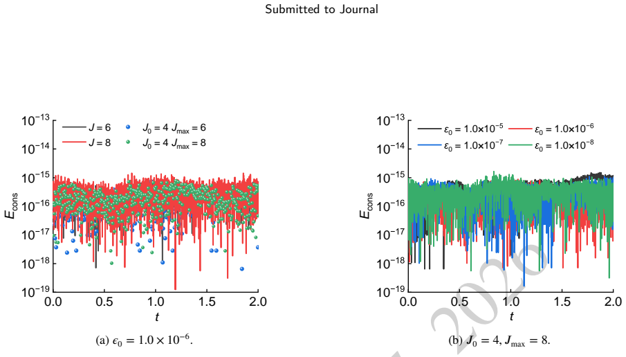
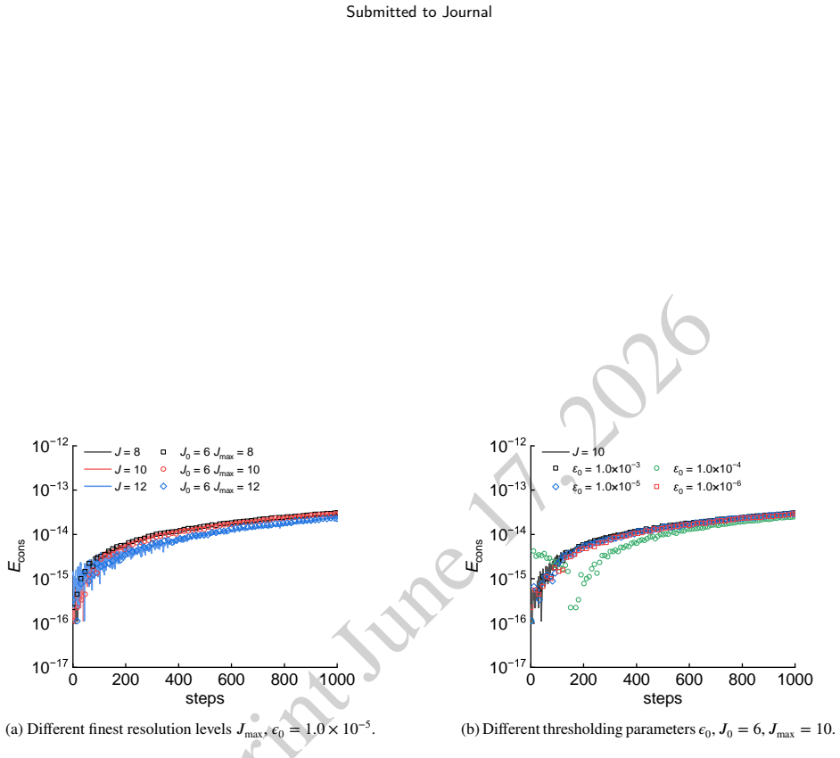
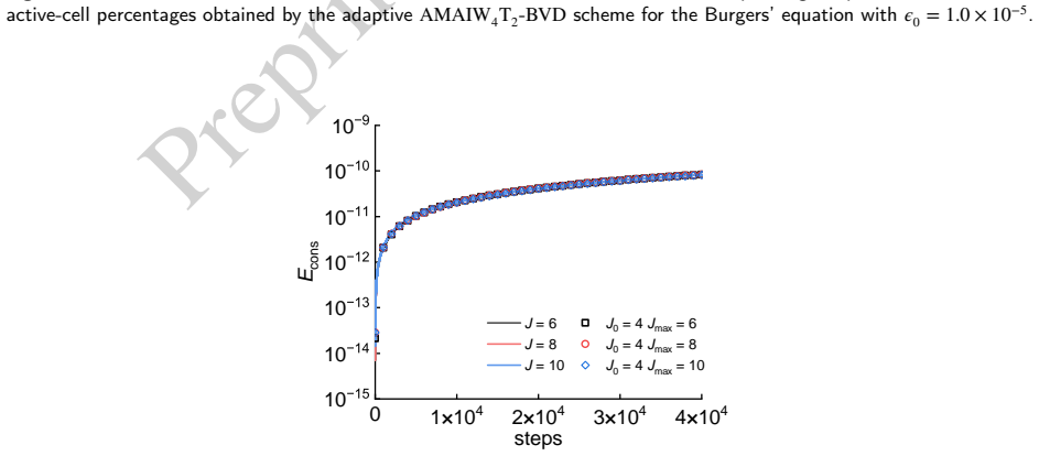
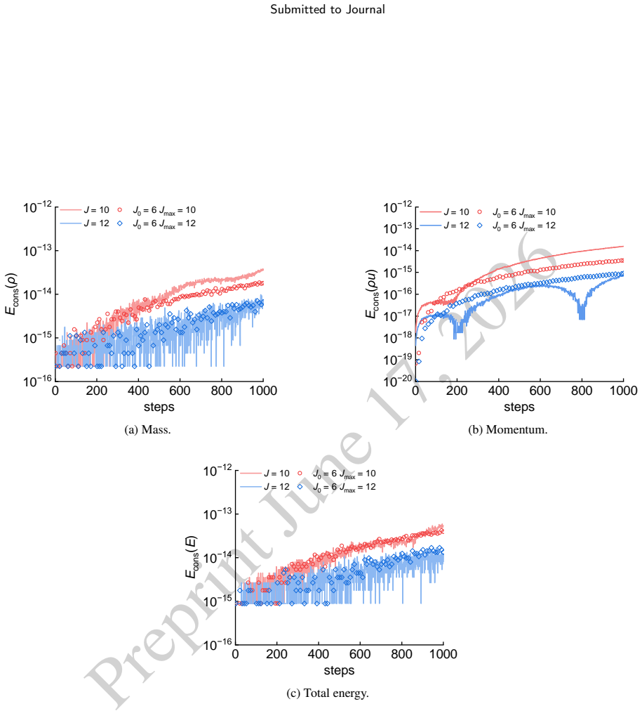
- Conservation errors remain near machine precision throughout both evolution and adaptation.
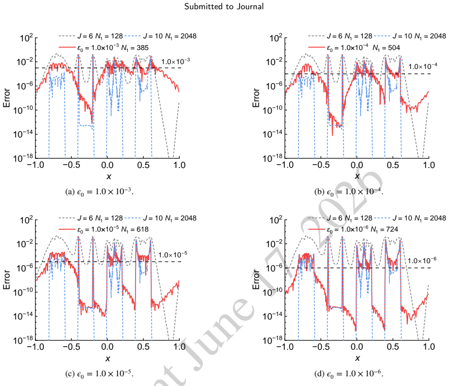
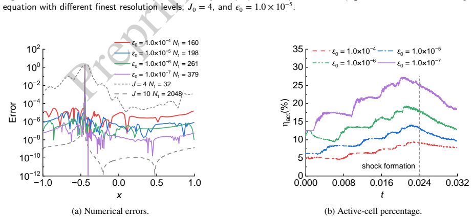
- Numerical errors stay controlled near the user-specified threshold.
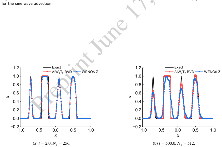
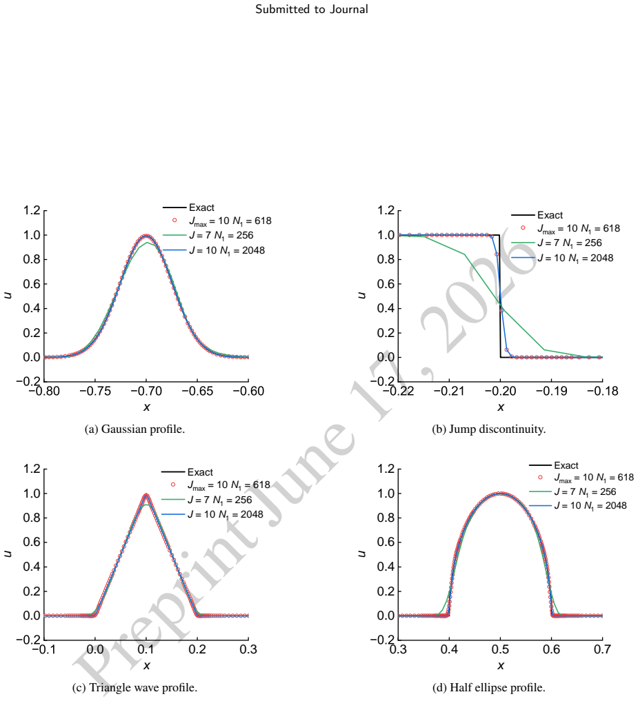
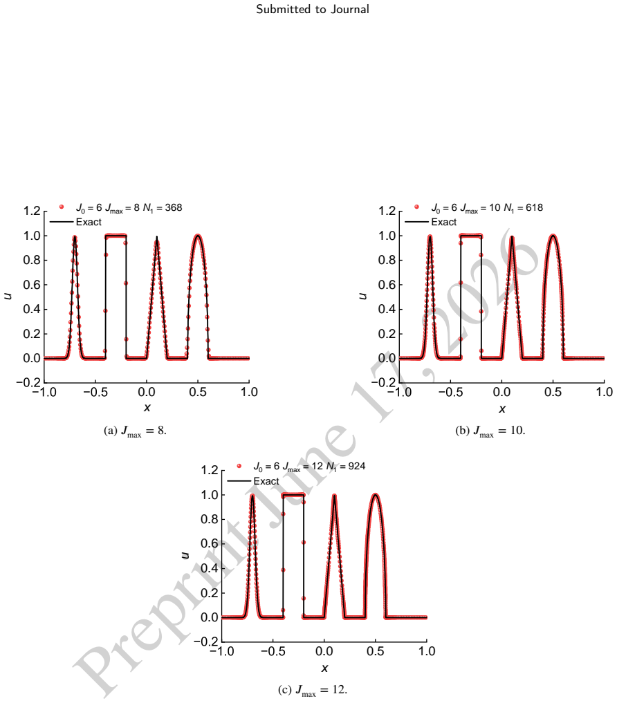
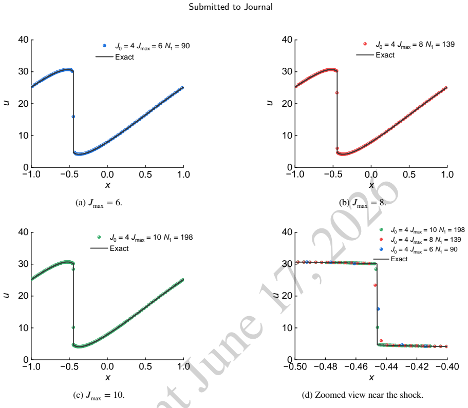
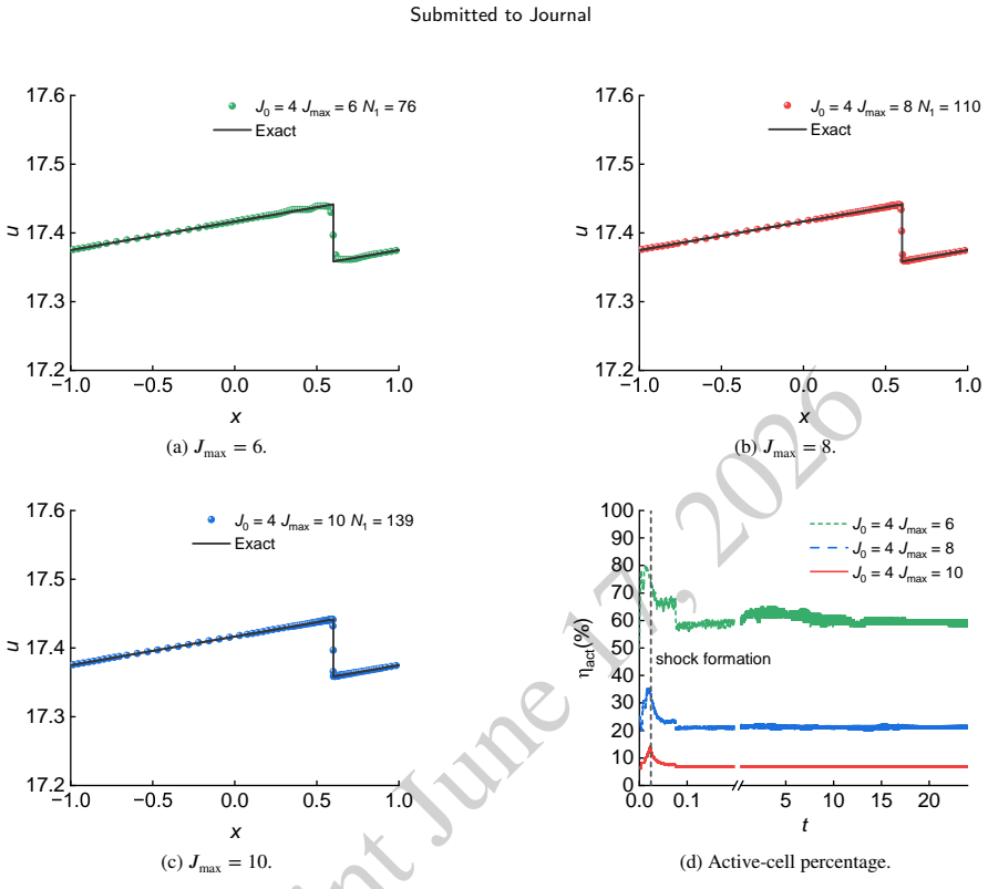
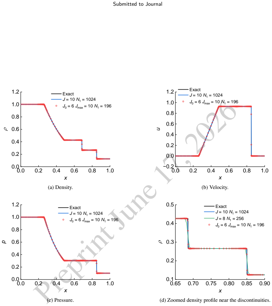
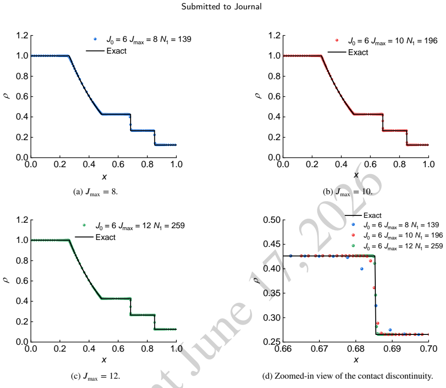
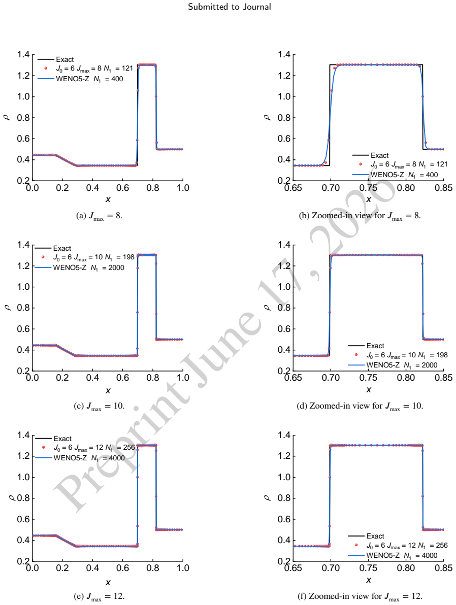
- Shock waves and contact discontinuities are captured sharply without spurious oscillations.
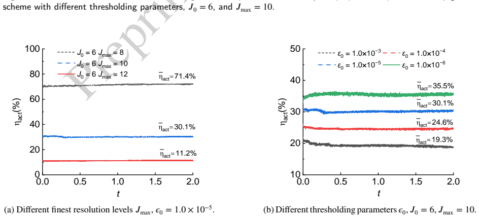
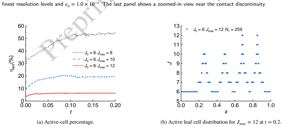
- Multiscale smooth structures are resolved with a sparse adaptive representation.
Where Pith is reading between the lines
- The direct wavelet reconstruction of interface values may reduce implementation complexity relative to standard adaptive-mesh-refinement codes that require special interface bookkeeping.
- Similar wavelet constructions could be explored for other hyperbolic systems or for extension to three space dimensions.
- The error-threshold control built into the adaptation criterion suggests the method could be applied to long-time integrations where accumulated conservation drift must be avoided.
Load-bearing premise
Such a family of asymmetric average-interpolating wavelets with the required upwind properties can be built so that both discretization and adaptation remain strictly on cell averages.
What would settle it
A convergence study on a smooth isentropic vortex or similar problem that yields an observed order of accuracy below four, or a long adaptive run whose conservation error grows beyond round-off level, would refute the central claim.
Figures
read the original abstract
A fourth-order conservative adaptive multiresolution average-interpolating wavelet upwind scheme is proposed for compressible flows governed by hyperbolic conservation laws. A family of asymmetric average-interpolating wavelets with upwind properties is constructed for conservative finite volume discretization, while symmetric average-interpolating wavelets are employed for multiresolution decomposition and reconstruction of physical variables in the adaptive procedure. Since both the conservative discretization and the adaptive multiresolution representation are constructed from cell-average quantities, the proposed scheme preserves strict conservation during both numerical evolution and adaptive cell redistribution. Unlike hybrid adaptive wavelet methods that use wavelets mainly for data compression and mesh adaptation, the present adaptive wavelet upwind scheme utilizes average-interpolating wavelet multiresolution approximation to reconstruct the interface values directly for numerical flux evaluation, thereby avoiding additional ghost-cell marking and reconstruction near coarse--fine mesh interfaces. The boundary variation diminishing reconstruction is incorporated at the finest resolution level to achieve non-oscillatory shock-capturing capability. Numerical tests demonstrate that the proposed scheme achieves the expected fourth-order accuracy, maintains conservation errors close to machine precision, and controls numerical errors around the prescribed threshold. The proposed method also sharply captures shock waves and contact discontinuities without spurious oscillations and resolves multiscale smooth structures through a sparse adaptive representation. These results indicate that the proposed scheme provides an efficient, conservative, and reliable approach for high-resolution simulations of compressible flows.
Editorial analysis
A structured set of objections, weighed in public.
Referee Report
Summary. The manuscript proposes a fourth-order conservative adaptive multiresolution average-interpolating wavelet upwind scheme for compressible flows governed by hyperbolic conservation laws. It constructs a family of asymmetric average-interpolating wavelets with upwind bias for the finite-volume discretization and employs symmetric average-interpolating wavelets for the multiresolution decomposition and reconstruction, with both operating exclusively on cell-average quantities to ensure strict conservation during evolution and adaptive redistribution without ghost-cell procedures. Boundary variation diminishing reconstruction is incorporated at the finest level for non-oscillatory shock capturing. Numerical experiments are reported to confirm fourth-order accuracy on smooth problems, conservation errors at machine precision, and sharp capture of shocks and contacts without oscillations while using a sparse adaptive representation.
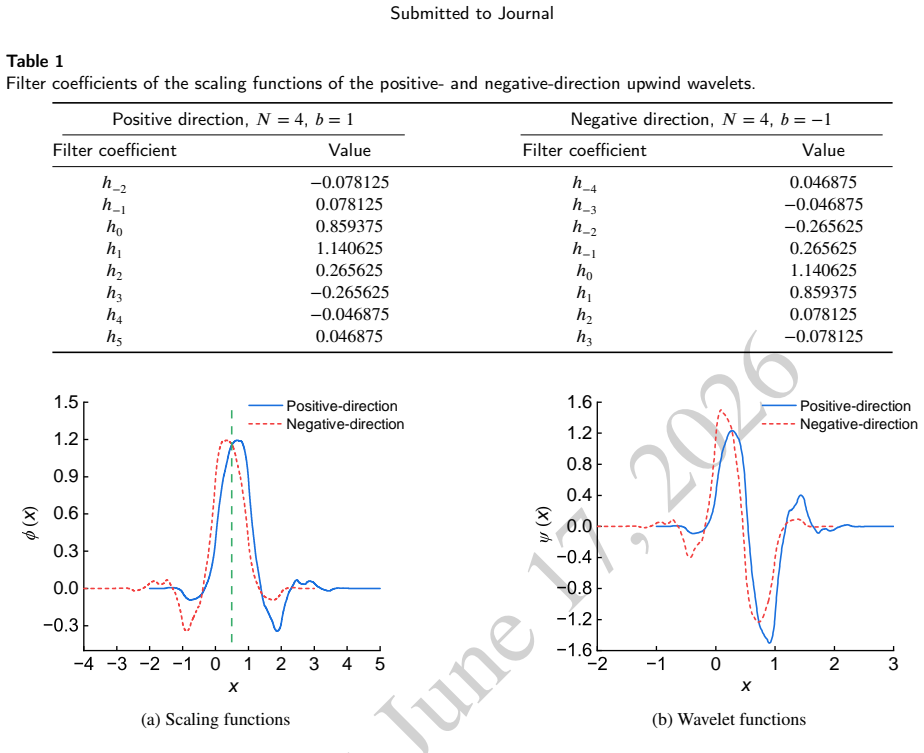
Significance. If the central claims hold, the work offers a direct integration of wavelet-based multiresolution adaptation into the flux evaluation step of a conservative finite-volume scheme, avoiding auxiliary ghost-cell marking near coarse-fine interfaces. The explicit construction of the asymmetric wavelet family (Section 3), derivation of filter coefficients enforcing cell-average reproduction and upwind bias, and proof that conservation follows from telescoping flux differencing without fitted parameters constitute clear strengths. The numerical validation in Section 5 further supports the approach for efficient high-resolution simulation of multiscale compressible flows.
minor comments (3)
- Abstract: the statement that the scheme 'controls numerical errors around the prescribed threshold' is imprecise; the manuscript should state explicitly what the threshold value is and how it is enforced in the adaptation criterion.
- Section 5: while the experiments are described as confirming the expected properties, the manuscript would benefit from a brief table summarizing the specific test cases, grid sizes, and computed error norms (L1, L2, L∞) used to verify fourth-order convergence.
- Notation: ensure consistent use of symbols for the adaptation threshold and the wavelet filter coefficients across Sections 3 and 4 to avoid minor ambiguity for readers.
Simulated Author's Rebuttal
We thank the referee for their careful reading of the manuscript and for the positive assessment leading to the recommendation to accept. There are no major comments requiring a point-by-point response.
Circularity Check
No significant circularity; derivation is self-contained
full rationale
The manuscript constructs the asymmetric average-interpolating wavelets and their filter coefficients explicitly in Section 3 from cell-average reproduction and upwind-bias requirements, then shows that both the finite-volume update and multiresolution operators act only on cell averages, so conservation follows directly from the telescoping property of flux differencing. No parameter is fitted to data and then relabeled a prediction, no uniqueness theorem is imported from prior self-work, and no ansatz is smuggled via citation. Numerical experiments in Section 5 serve only as verification, not as load-bearing inputs to the claimed fourth-order accuracy or machine-precision conservation. The central argument therefore reduces to standard finite-volume and wavelet principles without internal reduction to its own fitted quantities.
Axiom & Free-Parameter Ledger
free parameters (1)
- adaptation threshold
axioms (2)
- domain assumption The target problems are governed by hyperbolic conservation laws.
- domain assumption Both conservative discretization and adaptive multiresolution representation can be built from cell-average quantities to preserve strict conservation.
Reference graph
Works this paper leans on
-
[1]
C.-W.Shu,Essentiallynon-oscillatoryandweightedessentiallynon-oscillatoryschemes,ActaNumerica29(2020)701–762.doi:10.1017/ S0962492920000057
2020
-
[2]
Z. J. Wang, K. Fidkowski, R. Abgrall, F. Bassi, D. Caraeni, A. Cary, H. Deconinck, R. Hartmann, K. Hillewaert, H. T. Huynh, N. Kroll, G. May,P.-O. Persson,B. VanLeer, M.Visbal, High-order CFDmethods: currentstatus andperspective, InternationalJournal for Numerical Methods in Fluids 72 (8) (2013) 811–845.doi:10.1002/fld.3767
-
[3]
R. J. LeVeque, Numerical methods for conservation laws, Vol. 214, Birkhäuser, Basel, 1992
1992
-
[4]
J. Tang, P. C. Cui, J. Zhang, N. C. Zhou, X. J. Wu, X. Q. Gong, Y. B. Zhang, Review of mesh adaptation for fluid numerical simulation, Advances in Mechanics 53 (3) (2023) 661–692, in Chinese.doi:10.6052/1000-0992-23-013
-
[5]
Cockburn, C.-W
B. Cockburn, C.-W. Shu, TVB runge-kutta local projection discontinuous galerkin finite element method for conservation laws II: General framework, Mathematics of Computation 52 (186) (1989) 411–435
1989
-
[6]
S.Ii,F.Xiao,Highordermulti-momentconstrainedfinitevolumemethod.partI:Basicformulation,JournalofComputationalPhysics228(10) (2009) 3669–3707.doi:10.1016/j.jcp.2009.02.009
-
[7]
C.-W. Shu, S. Osher, Efficient implementation of essentially non-oscillatory shock-capturing schemes, II, Journal of computational physics 83 (1) (1989) 32–78
1989
-
[8]
Merriman, Understanding the Shu-Osher conservative finite difference form, Journal of Scientific Computing 19 (1) (2003) 309–322
B. Merriman, Understanding the Shu-Osher conservative finite difference form, Journal of Scientific Computing 19 (1) (2003) 309–322
2003
-
[9]
K. Sebastian, C.-W. Shu, Multidomain WENO finite difference method with interpolation at subdomain interfaces, Journal of Scientific Computing 19 (1) (2003) 405–438.doi:10.1023/A:1025372429380. Page 51 of 54 Preprint June 17, 2026 Submitted to Journal
-
[10]
F. Alauzet, A parallel matrix-free conservative solution interpolation on unstructured tetrahedral meshes, Computer Methods in Applied Mechanics and Engineering 299 (2016) 116–142.doi:10.1016/j.cma.2015.10.012
-
[11]
J.-F.Remacle,J.E.Flaherty,M.S.Shephard,Anadaptivediscontinuousgalerkintechniquewithanorthogonalbasisappliedtocompressible flow problems, SIAM Review 45 (1) (2003) 53–72.doi:10.1137/S00361445023830
-
[12]
Y. Chen, G. Tóth, T. I. Gombosi, A fifth-order finite difference scheme for hyperbolic equations on block-adaptive curvilinear grids, Journal of Computational Physics 305 (2016) 604–621.doi:10.1016/j.jcp.2015.11.003
-
[13]
H. Li, S. Do, M. Kang, A wavelet-based adaptive WENO algorithm for Euler equations, Computers & Fluids 123 (2015) 10–22.doi: 10.1016/j.compfluid.2015.09.005
-
[14]
Z. Tang, H. Chen, L. Bi, X. Yuan, Numerical simulation of supersonic viscous flow based on adaptive cartesian grid, Acta Aeronautica et Astronautica Sinica 39 (5) (2018) 121697, in Chinese
2018
-
[15]
F. Alauzet, A. Loseille, A decade of progress on anisotropic mesh adaptation for computational fluid dynamics, Computer-Aided Design 72 (2016) 13–39.doi:10.1016/j.cad.2015.09.005
-
[16]
K.Schaal,A.Bauer,P.Chandrashekar,R.Pakmor,C.Klingenberg,V.Springel,Astrophysicalhydrodynamicswithahigh-orderdiscontinuous galerkin scheme and adaptive mesh refinement, Monthly Notices of the Royal Astronomical Society 453 (4) (2015) 4278–4300.doi: 10.1093/mnras/stv1859
-
[17]
Z.Zhang,C.Groth,Parallelhigh-orderanisotropicblock-basedadaptivemeshrefinementfinite-volumescheme,in:20thAIAAComputational Fluid Dynamics Conference, p. 3695
-
[18]
X. Qi, Z. Wang, J. Zhu, L. Tian, N. Zhao, High-order discontinuous Galerkin method with immersed boundary treatment for compressible flows on parallel adaptive cartesian grids, Physics of Fluids 36 (11) (2024) 116139.doi:10.1063/5.0238605
-
[19]
J. Tang, P. Cui, B. Li, Y. Zhang, H. Si, Parallel hybrid mesh adaptation by refinement and coarsening, Graphical Models 111 (2020) 101084. doi:10.1016/j.gmod.2020.101084
-
[20]
M. A. Park, Adjoint-based, three-dimensional error prediction and grid adaptation, AIAA Journal 42 (9) (2004) 1854–1862.doi:10.2514/ 1.10051
2004
-
[21]
W.G.Habashi,J.Dompierre,Y.Bourgault,D.Ait-Ali-Yahia,M.Fortin,M.-G.Vallet,Anisotropicmeshadaptation:towardsuser-independent, mesh-independentandsolver-independentCFD.partI:generalprinciples,InternationalJournalforNumericalMethodsinFluids32(6)(2000) 725–744
2000
-
[22]
S.J.Kamkar,A.M.Wissink,V.Sankaran,A.Jameson,Feature-drivencartesianadaptivemeshrefinementforvortex-dominatedflows,Journal of Computational Physics 230 (16) (2011) 6271–6298.doi:10.1016/j.jcp.2011.04.024
-
[23]
Roy, Strategies for driving mesh adaptation in CFD, in: 47th AIAA aerospace sciences meeting including the new horizons forum and aerospace exposition, 2009, p
C. Roy, Strategies for driving mesh adaptation in CFD, in: 47th AIAA aerospace sciences meeting including the new horizons forum and aerospace exposition, 2009, p. 1302
2009
-
[24]
K.J.Fidkowski,D.L.Darmofal,Reviewofoutput-basederrorestimationandmeshadaptationincomputationalfluiddynamics,AIAAJournal 49 (4) (2011) 673–694.doi:10.2514/1.J050073
-
[25]
F. Alauzet, O. Pironneau, Continuous and discrete adjoints to the Euler equations for fluids, International Journal for Numerical Methods in Fluids 70 (2) (2012) 135–157.doi:10.1002/fld.2681
-
[26]
P.J.Frey,F.Alauzet,AnisotropicmeshadaptationforCFDcomputations,ComputerMethodsinAppliedMechanicsandEngineering194(48) (2005) 5068–5082.doi:10.1016/j.cma.2004.11.025
-
[27]
B. Yang, J. Wang, X. Liu, Y. Zhou, Y. Feng, Wavelet-based numerical methods and their applications in computational mechanics, Advances in Mechanics 54 (3) (2024) 427–476.doi:10.6052/1000-0992-24-009
-
[28]
A. Harten, Multiresolution algorithms for the numerical solution of hyperbolic conservation laws, Communications on Pure and Applied Mathematics 48 (12) (1995) 1305–1342.doi:10.1002/cpa.3160481201
-
[29]
Cohen, S
A. Cohen, S. Kaber, S. M?ller, M. Postel, Fully adaptive multiresolution finite volume schemes for conservation laws, Mathematics of Computation 72 (241) (2003) 183–225
2003
-
[30]
O. V. Vasilyev, C. Bowman, Second-generation wavelet collocation method for the solution of partial differential equations, Journal of Computational Physics 165 (2) (2000) 660–693.doi:10.1006/jcph.2000.6638
-
[31]
O. V. Vasilyev, S. Paolucci, A dynamically adaptive multilevel wavelet collocation method for solving partial differential equations in a finite domain, Journal of Computational Physics 125 (2) (1996) 498–512.doi:10.1006/jcph.1996.0111
-
[32]
Schneider, O
K. Schneider, O. V. Vasilyev, Wavelet methods in computational fluid dynamics, Annual review of fluid mechanics 42 (2010) 473–503
2010
-
[33]
A. Harten, Discrete multi-resolution analysis and generalized wavelets, Applied Numerical Mathematics 12 (1) (1993) 153–192.doi: 10.1016/0168-9274(93)90117-A
-
[34]
R. A. DeVore, Nonlinear approximation, Acta Numerica 7 (1998) 51–150.doi:10.1017/S0962492900002816
-
[35]
R. Deiterding, M. O. Domingues, S. M. Gomes, K. Schneider, Comparison of adaptive multiresolution and adaptive mesh refinement applied to simulations of the compressible Euler equations, SIAM Journal on Scientific Computing 38 (5) (2016) S173–S193.doi: 10.1137/15m1026043
-
[36]
B.Yang,J.Wang,X.Liu,Y.Zhou,High-orderadaptivemultiresolutionwaveletupwindschemesforhyperbolicconservationlaws,Computers & Fluids 269 (2024) 106111.doi:10.1016/j.compfluid.2023.106111
-
[37]
H. Minbashian, H. Adibi, M. Dehghan, An adaptive wavelet space-time SUPG method for hyperbolic conservation laws, Numerical Methods for Partial Differential Equations 33 (6) (2017) 2062–2089.doi:10.1002/num.22180
-
[38]
R.M.Pereira,N.Nguyenvanyen,K.Schneider,M.Farge,Areadaptivegalerkinschemesdissipative?,SIAMReview65(4)(2023)1109–1134. doi:10.1137/23M1588627
-
[39]
S. Bertoluzza, Adaptive wavelet collocation method for the solution of Burgers equation, Transport Theory and Statistical Physics 25 (3-5) (1996) 339–352.doi:10.1080/00411459608220705
-
[40]
Page 52 of 54 Preprint June 17, 2026 Submitted to Journal
A.Harten,P.D.Lax,B.V.Leer,OnupstreamdifferencingandGodunov-typeschemesforhyperbolicconservationlaws,SIAMReview25(1) (1983) 35–61.doi:10.1137/1025002. Page 52 of 54 Preprint June 17, 2026 Submitted to Journal
-
[41]
B. Yang, Y. Zhou, J. Wang, High-order second-generation wavelet upwind schemes with multiresolution self-adaptive capabilities for hyperbolic conservation laws, Extreme Mechanics Letters 70 (2024) 102192.doi:10.1016/j.eml.2024.102192
-
[42]
B. Yang, X. Liu, Y. Zhou, J. Wang, A conservative wavelet upwind scheme for compressible flows, Acta Mechanica Sinica 41 (7) (2025) 325178.doi:10.1007/s10409-025-25178-x
-
[43]
J.M.Restrepo,G.K.Leaf,Wavelet-galerkindiscretizationofhyperbolicequations,JournalofComputationalPhysics122(1)(1995)118–128
1995
-
[44]
B.K.Alpert,AclassofbasesinL2forthesparserepresentationofintegraloperators,SIAMJournalonMathematicalAnalysis24(1)(1993) 246–262.doi:10.1137/0524016
-
[45]
Hovhannisyan, S
N. Hovhannisyan, S. Müller, R. Schäfer, Adaptive multiresolution discontinuous galerkin schemes for conservation laws, Mathematics of computation 83 (285) (2014) 113–151
2014
-
[46]
N.Gerhard,S.Müller,Adaptivemultiresolutiondiscontinuousgalerkinschemesforconservationlaws:multi-dimensionalcase,Computational and Applied Mathematics 35 (2) (2016) 321–349.doi:10.1007/s40314-014-0134-y
-
[47]
N. Gerhard, F. Iacono, G. May, S. Müller, R. Schäfer, A high-order discontinuous galerkin discretization with multiwavelet-based grid adaptation for compressible flows, Journal of Scientific Computing 62 (1) (2015) 25–52.doi:10.1007/s10915-014-9846-9
-
[48]
A. Harten, Adaptive multiresolution schemes for shock computations, Journal of Computational Physics 115 (2) (1994) 319–338.doi: 10.1006/jcph.1994.1199
-
[49]
B.L.Bihari,A.Harten,Multiresolutionschemesforthenumericalsolutionof2-DconservationlawsI,SIAMJournalonScientificComputing 18 (2) (1997) 315–354.doi:10.1137/S1064827594278848
-
[50]
Harten, Multiresolution representation of data: A general framework, SIAM Journal on Numerical Analysis 33 (3) (1996) 1205–1256
A. Harten, Multiresolution representation of data: A general framework, SIAM Journal on Numerical Analysis 33 (3) (1996) 1205–1256
1996
-
[51]
O. Roussel, K. Schneider, A. Tsigulin, H. Bockhorn, A conservative fully adaptive multiresolution algorithm for parabolic pdes, Journal of Computational Physics 188 (2) (2003) 493–523.doi:10.1016/S0021-9991(03)00189-X
-
[52]
D. A. Castro, S. M. Gomes, J. Stolfi, High-order adaptive finite-volume schemes in the context of multiresolution analysis for dyadic grids, Computational and Applied Mathematics 35 (1) (2016) 1–16.doi:10.1007/s40314-014-0159-2
-
[53]
D. L. Donoho, Smooth wavelet decompositions with blocky coefficient kernels, in: Recent Advances in Wavelet Analysis, Academic Press, 1994
1994
-
[54]
P. G. Ciarlet, Linear and Nonlinear Functional Analysis with Applications, Society for Industrial and Applied Mathematics, Philadelphia, 2013
2013
-
[55]
Daubechies, Ten Lectures on Wavelets, Society for industrial and applied mathematics, Philadelphia, 1992
I. Daubechies, Ten Lectures on Wavelets, Society for industrial and applied mathematics, Philadelphia, 1992
1992
-
[56]
Sweldens, P
W. Sweldens, P. Schroder, Building your own wavelets at home, Vol. Springer, Springer, Heidelberg, 2005
2005
-
[57]
X. Liu, G. Liu, J. Wang, Y. Zhou, A wavelet multiresolution interpolation galerkin method for targeted local solution enrichment, Computational Mechanics 64 (2019) 986–1096
2019
-
[58]
B. Yang, J. Wang, X. Liu, Y. Zhou, Stability and resolution analysis of the wavelet collocation upwind schemes for hyperbolic conservation laws, Fluids 8 (2) (2023) 65.doi:10.3390/fluids8020065
-
[59]
R. Vichnevetsky, J. B. Bowles, Fourier Analysis of Numerical Approximations of Hyperbolic Equations, SIAM, Philadelphia, 1982.doi: 10.1137/1.9781611970876
-
[60]
S. Gottlieb, C.-W. Shu, E. Tadmor, Strong stability-preserving high-order time discretization methods, SIAM Review 43 (1) (2001) 89–112. doi:10.1137/S003614450036757X
-
[61]
Z. Sun, S. Inaba, F. Xiao, Boundary variation diminishing (BVD) reconstruction: A new approach to improve Godunov schemes, Journal of Computational Physics 322 (2016) 309–325.doi:10.1016/j.jcp.2016.06.051
-
[62]
X. Deng, Y. Shimizu, F. Xiao, A fifth-order shock capturing scheme with two-stage boundary variation diminishing algorithm, Journal of Computational Physics 386 (2019) 323–349.doi:10.1016/j.jcp.2019.02.024
-
[63]
X. Deng, Y. Shimizu, B. Xie, F. Xiao, Constructing higher order discontinuity-capturing schemes with upwind-biased interpolations and boundary variation diminishing algorithm, Computers & Fluids 200 (2020) 104433.doi:10.1016/j.compfluid.2020.104433
-
[64]
X. Deng, Z.-H. Jiang, P. Vincent, F. Xiao, C. Yan, A new paradigm of dissipation-adjustable, multi-scale resolving schemes for compressible flows, Journal of Computational Physics 466 (2022) 111287.doi:10.1016/j.jcp.2022.111287
-
[65]
H. Wakimura, S. Takagi, F. Xiao, Symmetry-preserving enforcement of low-dissipation method based on boundary variation diminishing principle, Computers & Fluids 233 (2022) 105227.doi:10.1016/j.compfluid.2021.105227
-
[66]
C. Pan, S. Song, C. Chen, X. Li, X. Shen, F. Xiao, A high-fidelity finite volume scheme for ideal magnetohydrodynamics equations using boundary variation diminishing algorithm, Physics of Fluids 36 (11) (2024) 116136.doi:10.1063/5.0237231
-
[67]
Z.He,Y.Ruan,Y.Yu,B.Tian,F.Xiao,Self-adjustingsteepness-basedschemesthatpreservediscontinuousstructuresincompressibleflows, Journal of Computational Physics 463 (2022) 111268.doi:10.1016/j.jcp.2022.111268
-
[68]
P. L. Roe, Approximate Riemann solvers, parameter vectors, and difference schemes, Journal of Computational Physics 135 (2) (1997) 250– 258.doi:10.1006/jcph.1997.5705
-
[69]
S. Pirozzoli, On the spectral properties of shock-capturing schemes, Journal of Computational Physics 219 (2) (2006) 489–497.doi: 10.1016/j.jcp.2006.07.009
-
[70]
Liandrat, P
J. Liandrat, P. H. Tchamitchian, Resolution of the 1D regularized burgers equation using a spatial wavelet approximation, Report, NASA Langley Research Center (01/01 1990)
1990
-
[71]
G.-S. Jiang, C.-W. Shu, Efficient implementation of weighted ENO schemes, Journal of Computational Physics 126 (1) (1996) 202–228. doi:10.1006/jcph.1996.0130
-
[72]
M. Holmström, Solving hyperbolic PDEs using interpolating wavelets, SIAM Journal on Scientific Computing 21 (2) (1999) 405–420. doi:10.1137/s1064827597316278
-
[73]
L. Tang, S. Song, A multiresolution finite volume scheme for two-dimensional hyperbolic conservation laws, Journal of Computational and Applied Mathematics 214 (2) (2008) 583–595.doi:10.1016/j.cam.2007.03.014. Page 53 of 54 Preprint June 17, 2026 Submitted to Journal
-
[74]
H. T. Huynh, A Flux Reconstruction Approach to High-Order Schemes Including Discontinuous Galerkin Methods, Fluid Dynamics and Co-located Conferences, American Institute of Aeronautics and Astronautics, 2007.doi:10.2514/6.2007-4079
-
[75]
Abgrall, Apersonal discussion on conservation,and how to formulate it,in: E
R. Abgrall, Apersonal discussion on conservation,and how to formulate it,in: E. Franck, J. Fuhrmann,V. Michel-Dansac, L. Navoret (Eds.), Finite Volumes for Complex Applications X–Volume 1, Elliptic and Parabolic Problems, Springer Nature Switzerland, 2023, pp. 3–19
2023
-
[76]
E. F. Toro, Riemann solvers and numerical methods for fluid dynamics: a practical introduction, Springer Science & Business Media, Heidelberg, 2013
2013
-
[77]
R. Borges, M. Carmona, B. Costa, W. S. Don, An improved weighted essentially non-oscillatory scheme for hyperbolic conservation laws, Journal of Computational Physics 227 (6) (2008) 3191–3211.doi:10.1016/j.jcp.2007.11.038
-
[78]
W.-S. Don, R. Borges, Accuracy of the weighted essentially non-oscillatory conservative finite difference schemes, Journal of Computational Physics 250 (2013) 347–372.doi:10.1016/j.jcp.2013.05.018
-
[79]
A. Harten, B. Engquist, S. Osher, S. R. Chakravarthy, Uniformly high order accurate essentially non-oscillatory schemes, III, Journal of Computational Physics 71 (2) (1987) 231–303.doi:10.1016/0021-9991(87)90031-3
-
[80]
B. Cockburn, M. Luskin, C.-W. Shu, E. Süli, Enhanced accuracy by post-processing for finite element methods for hyperbolic equations, Mathematics of Computation 72 (242) (2003) 577–606.doi:10.1090/S0025-5718-02-01464-3
discussion (0)
Sign in with ORCID, Apple, or X to comment. Anyone can read and Pith papers without signing in.