Patnaik-Pearson intrinsic dimension for internal representations of neural networks
Pith reviewed 2026-07-03 23:39 UTC · model grok-4.3
The pith
The Patnaik-Pearson dimension measures intrinsic dimension in neural network representations and aligns critical tail exponents with HTSR and SETOL when weight matrices follow Pareto spectra.
A machine-rendered reading of the paper's core claim, the machinery that carries it, and where it could break.
Core claim
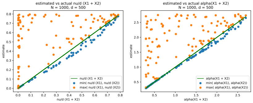
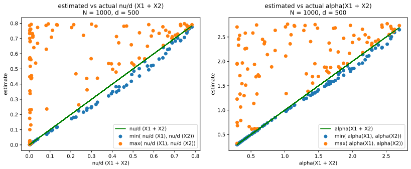
For weight matrices whose Empirical Spectral Density follows a Pareto distribution, the Patnaik-Pearson dimension relates directly to HTSR and SETOL analysis such that the critical values of the tail exponent coincide between the two approaches.
What carries the argument
The Patnaik-Pearson dimension, an intrinsic dimension estimator constructed from the TwoNN method combined with Patnaik-Pearson statistics, applied to weight matrices and token embeddings treated as data manifolds.
If this is right
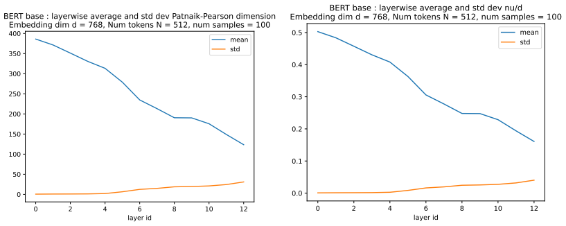
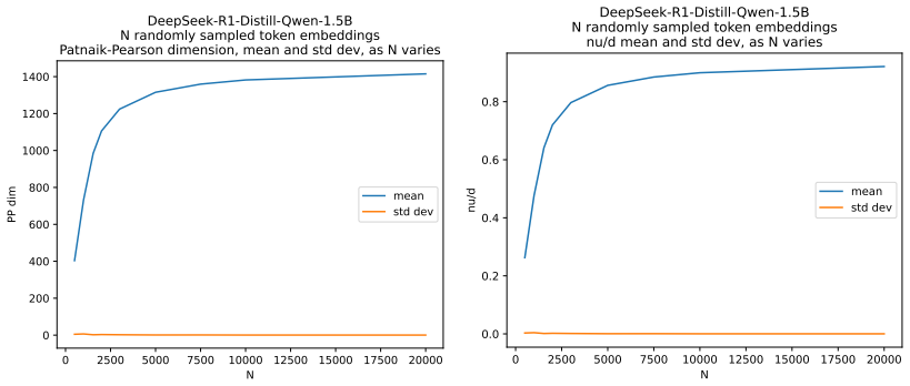
- The dimension of the initial token embedding manifold can be computed directly for transformer models.
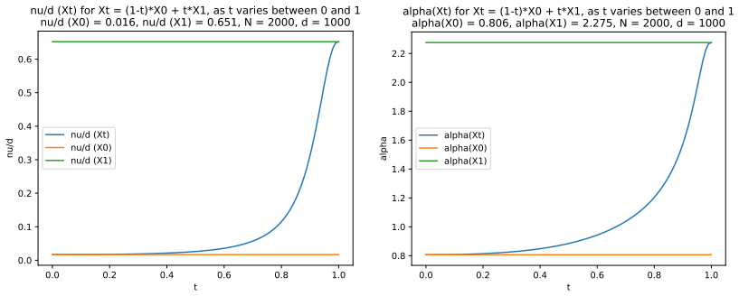
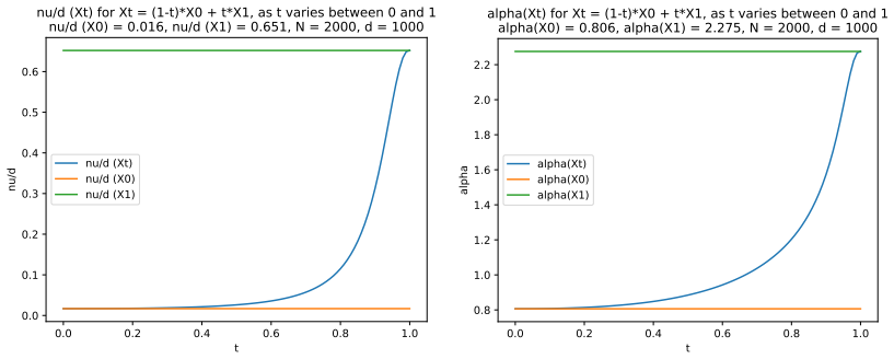
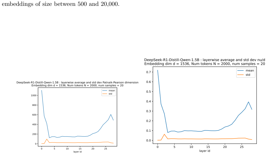
- The Patnaik-Pearson dimension evolves in measurable ways as embeddings pass through successive layers.
- The coincidence of critical tail exponents holds specifically under the Pareto assumption for spectral densities.
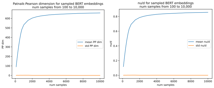
- Numerical evaluation on real models like BERT-base confirms the dimension can be tracked layer by layer.
Where Pith is reading between the lines
- If the dimension stabilizes or changes predictably across layers, it may indicate fixed points in how networks compress or expand manifolds.
- The approach could extend to other architectures by treating attention weights or activations as additional manifolds.
- Discrepancies in non-Pareto cases might highlight when spectral methods lose their direct connection to intrinsic dimension estimates.
Load-bearing premise
The empirical spectral density of the weight matrices follows a Pareto power-law distribution.
What would settle it
Empirical computation on a weight matrix whose spectral density deviates from Pareto form, showing that the Patnaik-Pearson critical tail exponent no longer matches the HTSR or SETOL value.
Figures


read the original abstract
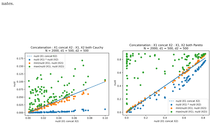
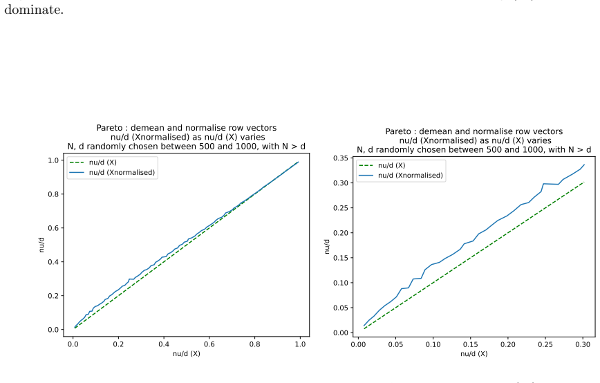
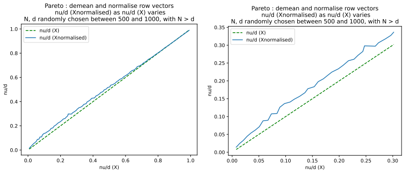
We define a new measure of intrinsic dimension of a data manifold, which we call the Patnaik-Pearson dimension, and apply this to internal representations of neural networks, in particular transformers. The inspiration for this comes from the HTSR and SETOL work of Martin, Mahoney and Hinrichs, combined with the TwoNN intrinsic dimension estimator of Facco et al. We prove various properties of this intrinsic dimension estimator. Treating weight matrices of neural networks as data manifolds, for weight matrices whose Empirical Spectral Density follows a Pareto (Power Law) distribution, we relate the Patnaik-Pearson dimension to the HTSR and SETOL analysis, and show that critical values of the tail exponent coincide for the two approaches. Using a combination of theoretical and numerical techniques, we study the behaviour of the Patnaik-Pearson dimension of a data manifold under the transformations typical to neural networks. We apply this machinery to the BERT-base and DeepSeek-R1-Distill-Qwen-1 models, to investigate first the Patnaik-Pearson dimension of the initial data manifold of token embeddings, and second the evolution of the Patnaik-Pearson dimension as token embeddings pass through the layers of the model. Code and notebooks used for the numerical results presented here is available at https://github.com/tdhadfield/PatnaikPearson
Editorial analysis
A structured set of objections, weighed in public.
Referee Report
Summary. The manuscript defines the Patnaik-Pearson intrinsic dimension estimator for data manifolds, drawing from HTSR/SETOL and the TwoNN method. It proves properties of the estimator, relates the dimension to HTSR/SETOL analysis specifically for weight matrices whose empirical spectral density follows a Pareto distribution (showing coincidence of critical tail exponents), examines the estimator's behavior under typical neural network transformations, and applies it to study token embeddings and their evolution through layers in BERT-base and DeepSeek-R1-Distill-Qwen-1 models. Code is provided for the numerical results.
Significance. If the conditional relation holds and the applications are robust, the work offers a new intrinsic dimension tool that connects to heavy-tailed spectral regularization frameworks, potentially aiding analysis of representation geometry in transformers. The explicit conditioning on the Pareto ESD and the availability of reproducible code are strengths.
minor comments (3)
- The abstract states that the relation to HTSR/SETOL holds for weight matrices with Pareto ESD, but the applications focus on token embeddings; clarify in the introduction or §3 whether the Pareto condition is checked or relevant for the BERT/DeepSeek experiments.
- The manuscript mentions proving 'various properties' of the estimator; ensure the main text explicitly lists these properties with references to the relevant theorems or propositions.
- Minor notation inconsistencies may exist between the Patnaik-Pearson definition and the TwoNN baseline; verify consistency in the methods section.
Simulated Author's Rebuttal
We thank the referee for the careful reading and positive assessment of the manuscript, including the recommendation for minor revision. No specific major comments are provided in the report, so there are no individual points to address point-by-point. We are happy to make any minor changes the editor may request based on the overall summary.
Circularity Check
No significant circularity; derivation self-contained
full rationale
The paper defines the Patnaik-Pearson dimension by combining the TwoNN estimator with concepts from HTSR/SETOL, proves independent properties of the new estimator, and derives the relation between critical tail exponents only conditionally on the explicit assumption that ESD follows a Pareto distribution. No step equates the new dimension to a fitted input or prior result by construction, and no self-citation chain is load-bearing for the central claims. The applications to BERT and DeepSeek are presented as separate empirical uses of the defined machinery.
Axiom & Free-Parameter Ledger
Reference graph
Works this paper leans on
-
[1]
Alessio Ansuini, Alessandro Laio, Jakob H. Macke, Davide Zoccolan,Intrinsic dimension of data representations in deep neural networks.https://arxiv.org/abs/1905.12784
-
[2]
Hari Bercovici, Vittorino Pata, Philippe Biane,Stable Laws and Domains of Attraction in Free Probability Theory.Annals of Mathematics, 1999-05, Vol.149 (3), p.1023-1060
1999
-
[3]
https://arxiv.org/abs/2312.14688
Nicolas Boull´ e, Alex Townsend,A Mathematical Guide to Operator Learning. https://arxiv.org/abs/2312.14688
-
[4]
Cizeau, J
P. Cizeau, J. P. Bouchaud,Theory of Levy matrices.Phys Rev E Stat Phys Plasmas Fluids Relat Interdiscip Topics. 1994 Sep, 50(3):1810-1822
1994
-
[5]
DeepSeek-AI,DeepSeek−R1: Incentivising Reasoning Capability in LLMs via Reinforcement Learn- ing.https://github.com/deepseek-ai/DeepSeek-R1/blob/main/DeepSeek R1.pdf https://huggingface.co/deepseek-ai/DeepSeek-R1-Distill-Qwen-1.5B
-
[6]
BERT: Pre-training of Deep Bidirectional Transformers for Language Understanding
Jacob Devlin, Ming-Wei Chang, Kenton Lee, Kristina Toutanova,BERT : Pre-Training of Deep Bidi- rectional Transformers for Language Understanding.Proceedings of NAACL-HLT 2019, Minneapolis, 2-7 June 2019, 4171-7186. https://arxiv.org/abs/1810.04805
work page internal anchor Pith review Pith/arXiv arXiv 2019
- [7]
-
[8]
Paul Embrechts, Claudia Kl¨ uppelberg, Thomas Mikosch,Modelling Extremal Events : for Insurance and Finance.Springer Berlin Heidelberg (2003)
2003
-
[9]
Facco, E., d’Errico, M., Rodriguez, A. et al.,Estimating the intrinsic dimension of datasets by a minimal neighborhood information.Sci Rep 7, 12140 (2017). https://doi.org/10.1038/s41598-017-11873-y https://www.nature.com/articles/s41598-017-11873-y
-
[10]
The Shape of Adversarial Influence: Characterizing LLM Latent Spaces with Persistent Homology
Aideen Fay, In´ es Garc´ ıa-Redondo, Qiquan Wang, Haim Dubossarsky, Anthea Monod,The Shape of Adversarial Influence: Characterizing LLM Latent Spaces with Persistent Homology. https://arxiv.org/abs/2505.20435
work page internal anchor Pith review Pith/arXiv arXiv
-
[11]
Testing the Manifold Hypothesis
Charles Fefferman, Sanjoy Mitter, Hariharan Narayanan,Testing the Manifold Hypothesis. https://arxiv.org/abs/1310.0425
work page internal anchor Pith review Pith/arXiv arXiv
- [12]
-
[13]
Sergey Foss, Dmitry Korshunov, Stan Zachary,An Introduction to Heavy-Tailed and Subexponential Distributions.Springer (2012)
2012
-
[14]
In: International Conference on Learning Representations (ICLR)
Yuri Gardinazzi, Giada Panerai, Karthik Viswanathan, Alessio Ansuini, Alberto Caz- zaniga, Matteo Biagetti,Persistent Topological Features in Large Language Models. https://arxiv.org/abs/2410.11042
-
[15]
https://arxiv.org/abs/2402.00949
Kaie Kubjas, Jiayi Li, Maximilian Wiesmann,Geometry of Polynomial Neural Networks. https://arxiv.org/abs/2402.00949
- [16]
-
[17]
https://arxiv.org/abs/2509.11088
Alexandros Grosdos, Elina Robeva, Maksym Zubkov,Algebraic geometry of rational neural networks. https://arxiv.org/abs/2509.11088
-
[18]
Frank E. Grubbs, Helen J. Coon, E. S. Pearson,On the Use of Patnaik Type Chi Approximations to the Range in Significance Tests.Biometrika, Vol. 53, No. 1/2 (Jun., 1966), pp. 248-252. https://doi.org/10.2307/2334073 https://www.jstor.org/stable/2334073
-
[19]
https://arxiv.org/abs/2204.08624
German Magai, Anton Ayzenberg,Topology and Geometry of Data Manifold in Deep Learning. https://arxiv.org/abs/2204.08624
- [20]
-
[21]
Martin,WeightWatcher.https://github.com/CalculatedContent/WeightWatcher
Charles H. Martin,WeightWatcher.https://github.com/CalculatedContent/WeightWatcher
-
[22]
Martin,A Spectral Renormalization-Group View of Learning
Charles H. Martin,A Spectral Renormalization-Group View of Learning. https://www.linkedin.com/posts/charlesmartin14 a-spectral-renormalization-group-view-of- ugcPost-7471078735861944321-jXs
-
[23]
Martin, Christopher Hinrichs,SETOL: A Semi-Empirical Theory of (Deep) Learning
Charles H. Martin, Christopher Hinrichs,SETOL: A Semi-Empirical Theory of (Deep) Learning. https://arxiv.org/abs/2507.17912
-
[24]
Traditional and Heavy-Tailed Self Regularization in Neural Network Models
Charles H. Martin, Michael W. Mahoney,Traditional and Heavy-Tailed Self Regularization in Neural Network Models.https://arxiv.org/abs/1901.08276
work page internal anchor Pith review Pith/arXiv arXiv 1901
- [25]
-
[26]
Thomas Mikosch, Olivier Wintenberger,Extreme Value Theory for Time Series Models with Power- Law Tails.Springer, 2024
2024
-
[27]
https://papers.ssrn.com/sol3/papers.cfm?abstract id=6073468
Miquel Noguer I Alonso,The Complete Mathematics of Transformers: A Rigorous Treatment with Full Derivations, Proofs, and Theoretical Foundations. https://papers.ssrn.com/sol3/papers.cfm?abstract id=6073468
- [28]
-
[29]
B.,The non-centralχ 2- and F-distributions and their application.Biometrika, 36(1/2) (1949), 202-232
Patnaik, P. B.,The non-centralχ 2- and F-distributions and their application.Biometrika, 36(1/2) (1949), 202-232. https://doi.org/10.2307/2332542 33
-
[30]
S.,Note on an approximation to the distribution of noncentralχ 2.Biometrika, 46(3/4), (1959) 364
Pearson, E. S.,Note on an approximation to the distribution of noncentralχ 2.Biometrika, 46(3/4), (1959) 364. https://doi.org/10.2307/2333533
-
[31]
Marc Potters, Jean-Philippe Bouchaud,A first course in Random Matrix Theory : for physicists, engineers and data scientists.Cambridge University Press (2021)
2021
-
[32]
Alethea Power, Yuri Burda, Harri Edwards, Igor Babuschkin, Vedant Misra,Grokking: Generaliza- tion Beyond Overfitting on Small Algorithmic Datasets.https://arxiv.org/abs/2201.02177
work page internal anchor Pith review Pith/arXiv arXiv
-
[33]
Hari K. Prakash, Charles H. Martin,Grokking and Generalization Collapse: Insights fromHTSR theory.https://arxiv.org/abs/2506.04434
- [34]
-
[35]
Ashish Vaswani, Noam Shazeer, Niki Parmar, Jakob Uszkoreit, Llion Jones, Aidan N. Gomez, Lukasz Kaiser, Illia Polosukhin,Attention Is All You Need.https://arxiv.org/abs/1706.03762
work page internal anchor Pith review Pith/arXiv arXiv
-
[36]
Voiculescu, K
D. Voiculescu, K. Dykema, A. Nica,Free random variables.CRM Monograph Series, No. 1, A.M.S., Providence, RI, 1992
1992
-
[37]
https://arxiv.org/abs/2007.02876
James Vuckovic, Aristide Baratin, Remi Tachet des Combes,A Mathematical Theory of Attention. https://arxiv.org/abs/2007.02876
-
[38]
Suppose we have a region inR d, containing random points with (uniform) densityρ
Nick Whiteley, Annie Gray, Patrick Rubin-Delanchy,Statistical exploration of the Manifold Hypoth- esis.https://arxiv.org/abs/2208.11665v3 8 Appendix : The TwoNN intrinsic dimension formula We derive the formulae given in [9] which we use in Section 2.3, in particular (9). Suppose we have a region inR d, containing random points with (uniform) densityρ. Th...
discussion (0)
Sign in with ORCID, Apple, or X to comment. Anyone can read and Pith papers without signing in.