Entropy Objectives in Markov Decision Processes
Pith reviewed 2026-06-26 13:57 UTC · model grok-4.3
The pith
Entropy objectives in MDPs reduce to convex programs for strategy synthesis.
A machine-rendered reading of the paper's core claim, the machinery that carries it, and where it could break.
Core claim
We present a sound and conditionally relatively complete method to verify and synthesize strategies for entropy objectives in MDPs. The main technical step exploits convex duality and invariant synthesis to reduce the non-linear objectives to convex programs while preserving the required guarantees for the class of MDPs considered.
What carries the argument
Reduction of non-linear entropy objectives to convex programs via convex duality combined with invariant synthesis
Load-bearing premise
The non-linear entropy objectives admit a reduction to convex programs and invariant synthesis that preserves soundness and conditional completeness for the class of MDPs considered.
What would settle it
An MDP instance in which a strategy satisfying the entropy objective exists but the synthesis procedure either fails to produce a strategy or produces one that violates the objective.
Figures
read the original abstract
We consider the problem of synthesizing control policies that enforce a concentration property on the state distributions of a stochastic system. We present a formalization of this problem in terms of synthesizing strategies for maintaining an entropy-based objective in Markov Decision Processes (MDPs). We first show that even relaxed versions of this problem are complexity-theoretically hard. We then present a sound and (conditionally) relatively complete method to verify and synthesize strategies for such entropy objectives. The main challenge is the non-linear nature of such objectives, and our approach addresses this by exploiting and combining ideas from convex duality and invariant synthesis. We also investigate the role of memory and randomization in ensuring entropy objectives. Finally, we implement our ideas to evaluate our approach empirically on a few illustrative benchmarks.
Editorial analysis
A structured set of objections, weighed in public.
Referee Report
Summary. The paper formalizes synthesizing strategies for entropy-based objectives in MDPs to enforce concentration properties on state distributions in stochastic systems. It establishes complexity-theoretic hardness for relaxed versions of the problem, then proposes a sound and conditionally relatively complete verification/synthesis method that reduces the non-linear objectives to convex programs via convex duality combined with invariant synthesis. The work also examines the roles of memory and randomization and reports empirical results on illustrative benchmarks.
Significance. If the reduction to convex programs is correct and preserves the claimed properties, the result would be a useful contribution to verification of MDPs with non-linear objectives, extending convex-optimization techniques in a targeted way. The hardness result and the explicit treatment of memory/randomization are clear strengths; the empirical evaluation on benchmarks provides initial evidence of practicality.
major comments (1)
- [§4] §4 (main theorem on soundness/conditional completeness): the reduction from non-linear entropy objectives to convex programs is central to the claim, yet the manuscript does not supply an explicit counter-example or boundary case showing where the invariant-synthesis step fails to preserve conditional completeness; a concrete example MDP where the method returns 'unknown' would strengthen the conditional-completeness statement.
minor comments (2)
- [Preliminaries] Preliminaries section: the definition of the entropy objective (Eq. 3) uses a non-standard normalization; adding a short remark comparing it to Shannon entropy would improve readability for readers outside the immediate sub-area.
- [Empirical evaluation] Empirical evaluation: Table 1 reports runtimes but omits the number of states/actions in each benchmark MDP; including these sizes would allow readers to assess scalability claims.
Simulated Author's Rebuttal
We thank the referee for the positive assessment of our manuscript and the constructive comment. We address the major comment below.
read point-by-point responses
-
Referee: [§4] §4 (main theorem on soundness/conditional completeness): the reduction from non-linear entropy objectives to convex programs is central to the claim, yet the manuscript does not supply an explicit counter-example or boundary case showing where the invariant-synthesis step fails to preserve conditional completeness; a concrete example MDP where the method returns 'unknown' would strengthen the conditional-completeness statement.
Authors: We thank the referee for this observation. The conditional completeness of our method (Theorem 4) is established under the assumption that the invariant synthesis procedure succeeds in discovering a suitable invariant when one exists. While the formal statement already delineates this boundary, we agree that an explicit example MDP illustrating a case in which the method returns 'unknown' would improve reader intuition regarding the practical limits of the approach. In the revised manuscript we will add a small, self-contained MDP example in Section 4 demonstrating such a boundary case, without altering the main theorems or proofs. revision: yes
Circularity Check
No significant circularity
full rationale
The paper's central claim is a sound and conditionally relatively complete verification/synthesis method for entropy objectives in MDPs, obtained by reducing the non-linear problem to convex programs combined with invariant synthesis via convex duality. This reduction relies on standard external techniques (convex duality, invariant synthesis) rather than self-definition, fitted parameters renamed as predictions, or load-bearing self-citations. The abstract and description contain no equations or steps that reduce by construction to their own inputs; the hardness result and empirical evaluation are presented as separate from the derivation. The derivation chain is self-contained against external benchmarks.
Axiom & Free-Parameter Ledger
Reference graph
Works this paper leans on
-
[1]
ACM, 2018. DOI: 10.1145/3209108.3209185. [AMTZ22] M. Anand, V. Murali, A. Trivedi, and M. Zamani.𝑘-inductive barrier certificates for stochas- tic systems. InProc. 25th ACM International Conference on Hybrid Systems: Computation and Control (HSCC), pages 12:1–12:11. ACM, 2022. DOI: 10.1145/3501710.3519532. [BCJ+23] K. Batz, M. Chen, S. Junges, B. L. Kamin...
-
[2]
DOI: 10.1109/TAC.2023.3341282. [GLS93] M. Grötschel, L. Lovász, and A. Schrijver.Geometric Algorithms and Combinatorial Opti- mization, volume 2 ofAlgorithms and Combinatorics. Springer Berlin Heidelberg, Berlin, Heidelberg, second corrected edition, 1993. DOI: 10.1007/978-3-642-78240-4. [GM15] M. Gario and A. Micheli. PySMT: a solver-agnostic library for...
-
[3]
DOI: 10.1145/380752.380839. [Vaz03] V. V. Vazirani.Approximation Algorithms. Springer, 2003. DOI: 10.1007/978-3-662-04565-7. [Vis21] N. K. Vishnoi.Algorithms for Convex Optimization. Cambridge University Press, 2021. DOI: 10.1017/9781108699211. [Wil97] A. J. Wilkie. Schanuel’s Conjecture and the Decidability of the Real Exponential Field. In B. T. Hart, A...
-
[4]
In Russian. English translation:Matekon13 (3) (1977) 25–45. 24 A A strong duality result for entropy In this section, we provide the proof of Proposition 10. As mentioned in Section 5, we need a strong duality result which is usually stated under the additional hypothesis that the feasible point𝑥 0 has all its entriesstrictlypositive (this is the version ...
arXiv 1977
-
[5]
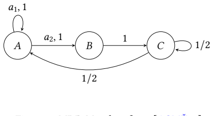
In this example, it is optimal to choose action𝑎 1 always
MDP𝑀 1 with 3 states, taken from running example of [ACMŽ23]) 𝐴 𝐵 𝐶 𝑎2,1 𝑎1,1 1 1/2 1/2 26 At the start, in𝜇 0, state A has probability 1 2, state B has probability 1 3, state C has probability 1 6. In this example, it is optimal to choose action𝑎 1 always. As the initial probability mass at𝐴 exceeds 1 𝑒 , any additional probability mass will only decreas...
-
[6]
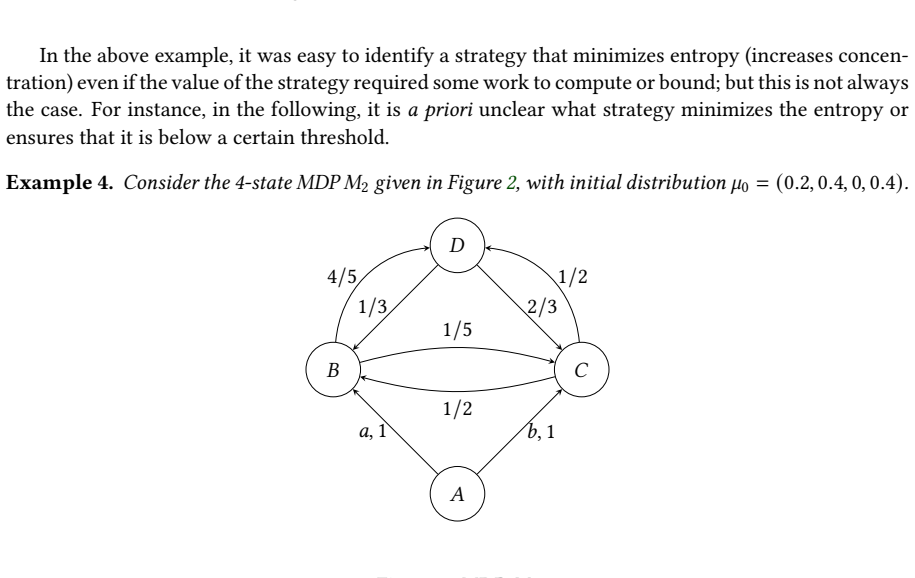
MDP𝑀 2 with 4 states: 3 1 2 0 𝑎,1 𝑏,1 4/5 1/5 1/2 1/2 1/3 2/3 The initial distribution𝜇 0 is (0.2, 0.4, 0, 0.4). •𝐾=0Starting from𝜇 0: The answer given by our Gurobi based solver (in a specific run) with an invariant set of size two is𝑒 𝐻(𝜇) =3.7568, with action𝑎being chosen with probability about 0.4. With a brute force computation, we can check that the...
1971
-
[7]
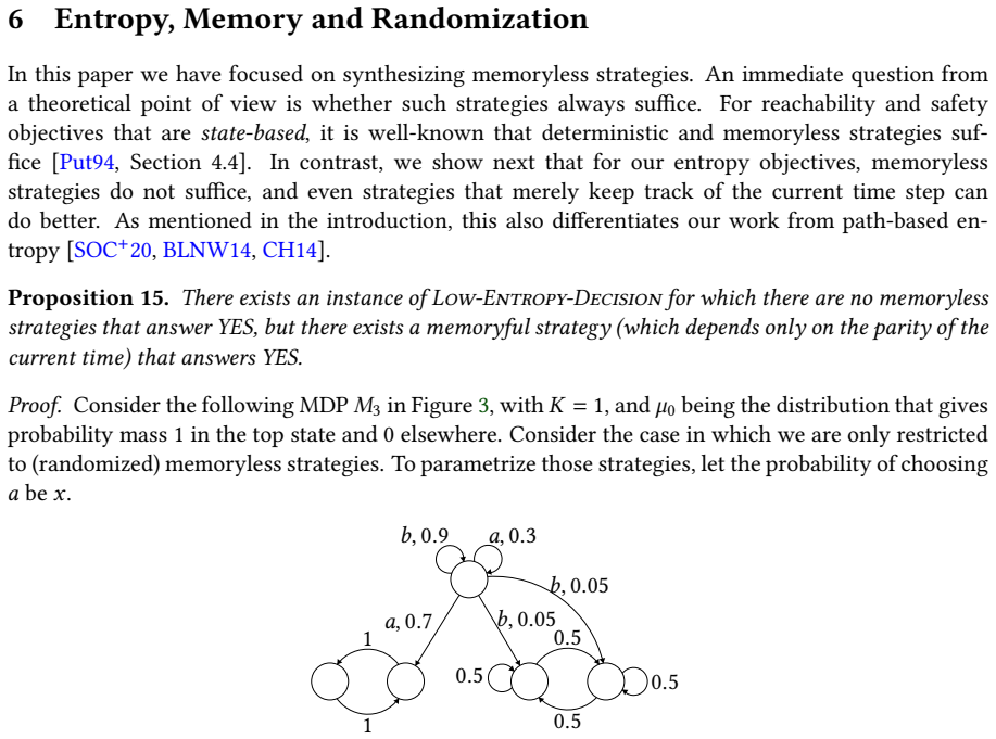
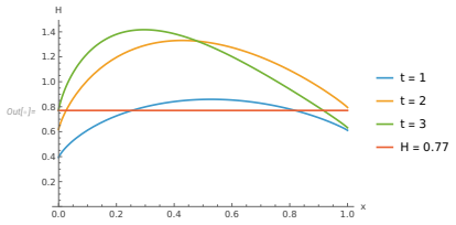
This is the same example as the one used in Proposition 15 above
A five-state MDP𝑀 3 with two bottom strongly connected component and a transient state. This is the same example as the one used in Proposition 15 above. 𝑎,0.71 1 0.5 0.5 0.5 0.5 𝑏,0.05 𝑏,0.05 𝑏,0.9 𝑎,0.3 At the start, i.e., in𝜇 0, the entire probability mass is in the top state. We can parameterize all memoryless strategies in terms of a single parameter...
-
[8]
•𝐾=2Starting from𝑀(𝜇 0,2): Our Gurobi based solver achieves a value of𝑒 𝐻(𝜇) of roughly 2.0, even with an invariant of size one
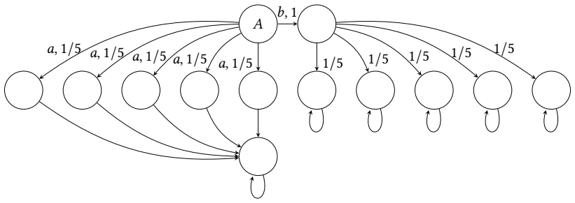
MDP𝑀 4 with 5 states and 2 actions : A B C D E 𝑎,1 𝑏,1 28 At the start, with𝜇 0 as state A has probability 9 10 and state E has probability 1 10. •𝐾=2Starting from𝑀(𝜇 0,2): Our Gurobi based solver achieves a value of𝑒 𝐻(𝜇) of roughly 2.0, even with an invariant of size one.. The optimal memoryless policy, in comparison, yields an answer of𝑒𝐻(𝜇) ≊1.35506, ...
-
[9]
With an invariant of size one, our Gurobi based tool reports an answer of𝑒 𝐻(𝜇) =2.9543, choosing action𝑎with probability one
MDP𝑀 5 with 3 states, with warm-up parameter𝐾=0: 𝐴 𝐵 𝐶 𝑎,1/2 𝑎,1/4 𝑎,1/4 𝑏,1/4 𝑏,1/4 𝑏,1/2 1/31/3 1/3 2/5 2/5 1/5 Initially, all the probability mass is in A, i.e.,𝜇 0 =(1,0,0). With an invariant of size one, our Gurobi based tool reports an answer of𝑒 𝐻(𝜇) =2.9543, choosing action𝑎with probability one. By a brute force computation we check that this is i...
-
[10]
Split (MDP with 4 states and 2 disconnected components taken from [ACMŽ23]): 𝐴 𝐵 𝐶 𝐷 𝑏,1 𝑎,0.9 𝑎,0.1 11 0.5 0.5 29 At the start, i.e., at𝜇0 =0, state A has probability 1 3 and state C has probability 2
-
[11]
Our Gurobi based solved reports an answer of about𝑒 𝐻(𝜇) =3.77976, with an invariant set of size one (𝐴+𝐵≤ 1 3), and the strategy of always choosing action𝑏
We consider the case where the warm-up parameter satisfies𝐾=0. Our Gurobi based solved reports an answer of about𝑒 𝐻(𝜇) =3.77976, with an invariant set of size one (𝐴+𝐵≤ 1 3), and the strategy of always choosing action𝑏. On simulating the MDP with this strategy, we find that the maximum entropy attained is at mostlog 3. However, under the restriction to c...
-
[12]
Note that all transition probabilities that are not labelled on edges are 1
Gridworld 1 (MDP with 8 states): This is a grid of size (2,4) with the point (0,1) being unreach- able, as shown in the figure with (0,0) being top-left and (1,3) being bottom-right. Note that all transition probabilities that are not labelled on edges are 1. Also there is a non-deterministic action at state (0,2), where one can go down or right, and a se...
-
[13]
At any other state, one of up to two actions - Down or Right - can be chosen, provided the action does not force one off the board or into an unreachable state
Gridworld 2 (MDP with 12 states): We have a grid of size (3,4) with the unreachable states as (1, 1), (2, 1) and (1, 3) (with(0,0)being top left and(2,3)the bottom right). At any other state, one of up to two actions - Down or Right - can be chosen, provided the action does not force one off the board or into an unreachable state. All transitions that are...
-
[14]
The initial distribution𝜇 0 is top-left state (0,0) having probability 1
From any reachable state except (2, 3) which does not have transitions marked in the figure, in the actual model there is a transition from that state to all other reachable states with uniform probability. The initial distribution𝜇 0 is top-left state (0,0) having probability 1. 30 Note again that while there is some randomness in this example, it is sim...
-
[15]
•𝐾=0Starting from𝜇 0: Our Gurobi based solver reports an answer of𝑒 𝐻(𝜇) =2.000, with an invariant set of size one
Markov chain𝑀𝐶1with two states BA 10.50.5 At the start, i.e., in𝜇 0, state A has probability 2 3 and state B has probability 1 3. •𝐾=0Starting from𝜇 0: Our Gurobi based solver reports an answer of𝑒 𝐻(𝜇) =2.000, with an invariant set of size one. By simulating a run of the MC, the maximum value of 𝑒𝐻 (𝜇)over the run is 1.88988. However, since the distribut...
-
[16]
•𝐾=1,2, starting from𝑀(𝜇 0,1)or𝑀(𝜇 0,2): Our Gurobi based solver outputs the correct optimal value of𝑒 𝐻(𝜇) =1.93782, with an invariant set of size two
Markov chain𝑀𝐶2with two states: A B 1 0.5 0.5 At the start, i.e., in𝜇 0, both A and B have 1 2 of the probability each. •𝐾=1,2, starting from𝑀(𝜇 0,1)or𝑀(𝜇 0,2): Our Gurobi based solver outputs the correct optimal value of𝑒 𝐻(𝜇) =1.93782, with an invariant set of size two. •𝐾=3, starting from𝑀(𝜇 0,3): Our Gurobi based solver outputs the correct optimal val...
-
[17]
Starting from𝜇 0 (𝐾=0), the Gurobi based solver reports the optimal answer of𝑒 𝐻(𝜇) =3
Markov chain MC3, an ergodic Markov chain with three states: 31 𝐴 𝐵 𝐶 0.5 0.25 0.25 0.5 0.25 0.25 0.25 0.25 0.5 Initially, the probability distribution𝜇 0 is (1, 0, 0). Starting from𝜇 0 (𝐾=0), the Gurobi based solver reports the optimal answer of𝑒 𝐻(𝜇) =3
-
[18]
body compartments
Insulin: Pharmokinetics benchmark taken originally from [CKV+11], but as modified in [AAGT15, Example 2], which we describe briefly. This Markov chain has five non-dummy nodes where three of the nodes correspond to the “body compartments” Plasma (Pl), Intersticial Fluid (IF), and “Utilization and degradation” (Ut). The node (Dr) models the drug being inje...
-
[19]
The optimal answer, obtained by simulating the Markov chain, is𝑒 𝐻(𝜇) =2.3717679
For this problem, starting from𝜇 0, the answer reported by our Gurobi based solver seems to depend quite significantly on the seed, with one particular run reporting the value𝑒 𝐻(𝜇) =2.72, obtained with an invariant of size five (for this example, it also helps to run the solver without the pre-imposed bounds on the magnitudes of the template variables). ...
-
[20]
Pagerank (A 5-state Markov chain taken from [AAGT15][Example 1, Fig 3.]). This chains has five states, with the transition matrix given by 1 80 19 60 3 40 19 60 67 2401 80 1 20 41 120 19 60 67 2401 16 1 4 3 8 1 4 1 161 80 1 20 7 8 1 20 1 8033 80 9 20 3 40 1 20 1 80 , with the rows and column corresponding to states A, B, C, D, and E ...
discussion (0)
Sign in with ORCID, Apple, or X to comment. Anyone can read and Pith papers without signing in.