Causal Variational Deep Embedding: A Family of Interventional Generators for Confounded Images
Pith reviewed 2026-06-26 14:07 UTC · model grok-4.3
The pith
A canonical class of augmented causal models with discrete cluster confounders is dense in Wasserstein distance for any diagram-compatible mechanism, allowing a mixture VAE to trace families of interventional image generators.
A machine-rendered reading of the paper's core claim, the machinery that carries it, and where it could break.
Core claim
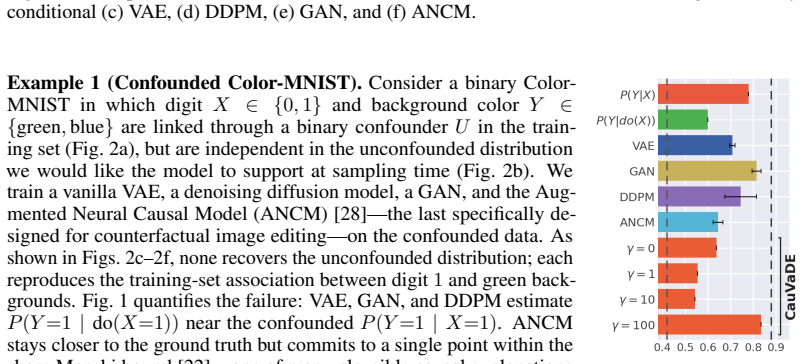
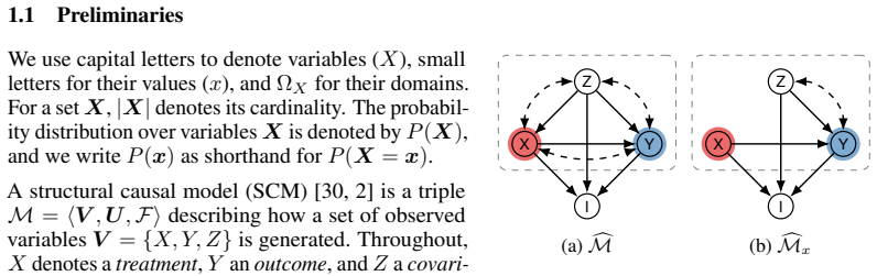
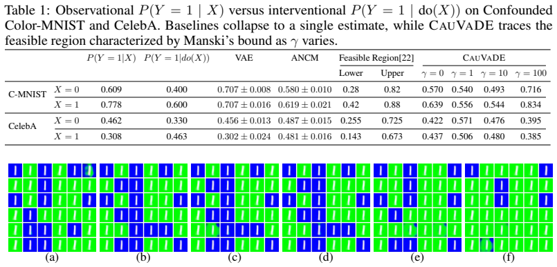
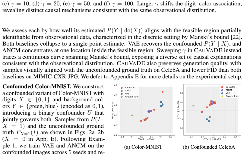
We prove that this canonical class is dense, in both observational and interventional Wasserstein distance, in the class of augmented SCMs compatible with a given causal diagram, and instantiate it as a mixture variational autoencoder whose cluster variable plays the role of the canonical confounder. An entropy regularizer with weight γ on the cluster posterior then traces a family of candidate causal effects that fit the observational data to comparable likelihood while spanning the feasible region.
What carries the argument
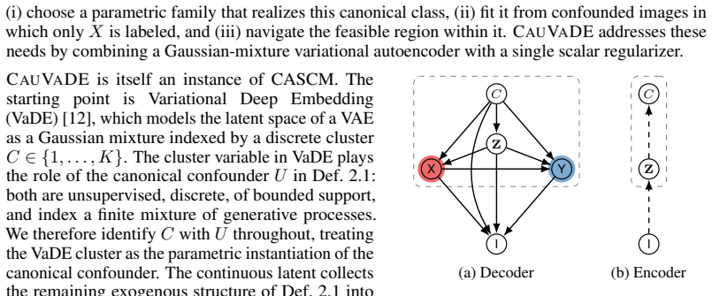
The canonical augmented SCM whose unobserved confounder is represented as a discrete latent cluster of bounded support, instantiated as a mixture variational autoencoder with entropy regularization on the cluster posterior.
If this is right
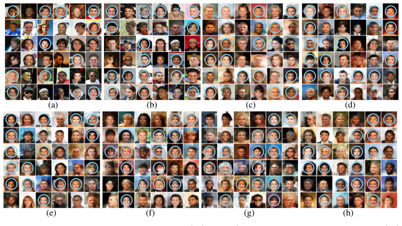
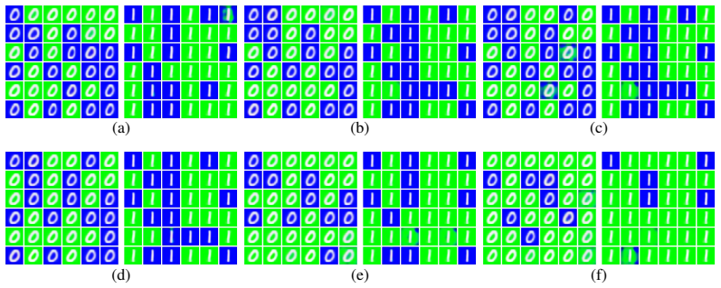
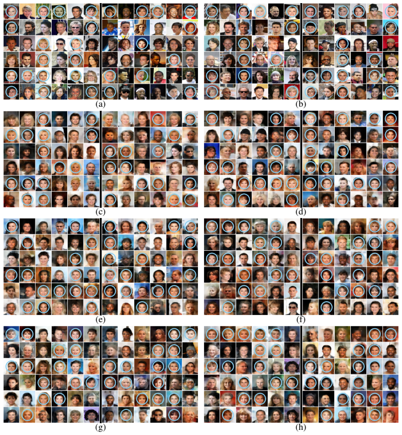
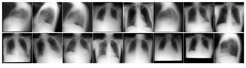
- The mixture VAE produces diverse interventional samples on image benchmarks.
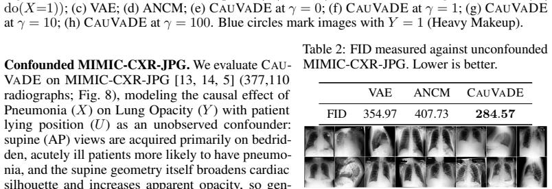
- The generated images achieve improved FID scores relative to an unconfounded reference.
- Varying the entropy weight γ yields a continuous family of causal effects that all match observational likelihood.
- The density result implies that the canonical form can stand in for any diagram-compatible model to arbitrary precision.
Where Pith is reading between the lines
- The same canonical reduction might be applied to non-image domains where confounders produce similar ambiguity in generative models.
- The regularization parameter γ offers a tunable control for the strength of the implied causal mechanism.
- Downstream tasks such as data augmentation or fairness auditing could use the spanned family to quantify sensitivity to confounding.
- Empirical checks on real confounded image pairs with known interventions would test whether the generated family brackets ground-truth effects.
Load-bearing premise
The unobserved confounder can be represented without loss of generality as a discrete latent cluster of bounded support, with all continuous variation absorbed into independent noise terms.
What would settle it
Construct a synthetic image dataset from a known augmented SCM with a continuous confounder, train the model, and check whether the interventional distributions obtained by varying γ include or approach the true interventional distribution in Wasserstein distance.
Figures
read the original abstract
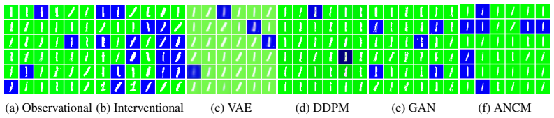
Deep generative models reproduce the observational distribution of their training data, inheriting any spurious associations it contains. A common source is an unobserved confounder that shapes both an attribute the user wants to control at sampling time and an attribute expected to vary in response. Existing causal generative approaches resolve the resulting ambiguity by imposing structural assumptions strong enough to single out one interventional distribution; in image domains, such assumptions are rarely warranted, and the data is generally consistent with a set of distinct causal mechanisms -- a feasible region of interventional distributions. We propose CauVaDE (Causal Variational Deep Embedding), built on a canonical augmented SCM in which the unobserved confounder collapses, without loss of generality, into a discrete latent cluster of bounded support while continuous variation is absorbed into independent noises. We prove that this canonical class is dense, in both observational and interventional Wasserstein distance, in the class of augmented SCMs compatible with a given causal diagram, and instantiate it as a mixture variational autoencoder whose cluster variable plays the role of the canonical confounder. An entropy regularizer with weight $\gamma$ on the cluster posterior then traces a family of candidate causal effects that fit the observational data to comparable likelihood while spanning the feasible region. Experiments on image data benchmarks show that CauVaDE produces diverse interventional samples and improves FID against an unconfounded reference.
Editorial analysis
A structured set of objections, weighed in public.
Referee Report
Summary. The paper proposes CauVaDE, a mixture variational autoencoder for generating interventional images under unobserved confounding. It defines a canonical augmented SCM in which the confounder is replaced by a discrete latent cluster variable of finite support (with continuous effects absorbed into independent noises), proves that this class is dense in both observational and interventional Wasserstein distance among all augmented SCMs compatible with a given causal diagram, and uses an entropy regularizer of weight γ on the cluster posterior to trace a family of candidate interventional distributions that fit the observational data while spanning the feasible region. Experiments on image benchmarks report improved FID scores relative to an unconfounded reference.
Significance. If the density result and the w.l.o.g. reduction hold, the work supplies a principled, assumption-light method for producing diverse interventional samples in image domains where multiple causal mechanisms remain consistent with the data; the entropy-regularized family explicitly parametrizes the feasible region rather than selecting a single effect. The combination of a provable approximation result with a practical VAE instantiation is a substantive contribution to causal generative modeling.
major comments (2)
- [Abstract; canonical augmented SCM definition and density proof] The central density claim rests on the assertion (abstract and canonical-SCM section) that any augmented SCM compatible with the diagram can be approximated arbitrarily closely by replacing the unobserved confounder with a discrete cluster of bounded support while pushing all remaining continuous variation into independent noises. This reduction is presented as without loss of generality, yet it is unclear whether interventional marginals are preserved when the confounder enters through non-separable continuous mechanisms; if the reduction fails for such diagrams, the spanned feasible region is strictly smaller than the true set and the density statement does not hold.
- [Entropy-regularizer paragraph; density theorem statement] The entropy regularizer is claimed to trace the feasible region independently of the specific fitted γ values. Without the explicit derivation showing that the Wasserstein distance to the target interventional distributions remains controlled uniformly in γ (or an explicit statement of the conditions under which this independence holds), it is impossible to confirm that the family genuinely spans the region rather than collapsing to a single point for some diagrams.
minor comments (2)
- [Experiments] The experimental section should report the precise range of γ values tested and the corresponding cluster-posterior entropy values to allow readers to verify that the reported FID improvements correspond to distinct points along the claimed family.
- [Model instantiation] Notation for the mixture components and the role of the cluster variable as the canonical confounder should be introduced with an explicit diagram or equation reference in the model section to improve readability.
Simulated Author's Rebuttal
We thank the referee for the constructive comments. We address each major point below.
read point-by-point responses
-
Referee: [Abstract; canonical augmented SCM definition and density proof] The central density claim rests on the assertion (abstract and canonical-SCM section) that any augmented SCM compatible with the diagram can be approximated arbitrarily closely by replacing the unobserved confounder with a discrete cluster of bounded support while pushing all remaining continuous variation into independent noises. This reduction is presented as without loss of generality, yet it is unclear whether interventional marginals are preserved when the confounder enters through non-separable continuous mechanisms; if the reduction fails for such diagrams, the spanned feasible region is strictly smaller than the true set and the density statement does not hold.
Authors: The canonical construction absorbs any continuous non-separable effects of the confounder into the independent noise terms by definition, so that the discrete cluster approximates the marginal distribution of the confounder while the SCM structure (and therefore the interventional marginals) is preserved. The density theorem then shows that the resulting class is dense in Wasserstein distance for both observational and interventional measures over all augmented SCMs compatible with the diagram. We will insert a short clarifying sentence in the canonical-SCM section of the revision to make this absorption step explicit for non-separable mechanisms. revision: yes
-
Referee: [Entropy-regularizer paragraph; density theorem statement] The entropy regularizer is claimed to trace the feasible region independently of the specific fitted γ values. Without the explicit derivation showing that the Wasserstein distance to the target interventional distributions remains controlled uniformly in γ (or an explicit statement of the conditions under which this independence holds), it is impossible to confirm that the family genuinely spans the region rather than collapsing to a single point for some diagrams.
Authors: Different values of γ produce posteriors with different entropies and therefore different effective cluster assignments, each of which corresponds to a distinct interventional distribution inside the feasible region while remaining observationally consistent. Because every such model lies inside the dense canonical class, the Wasserstein distance to any target interventional distribution is controlled uniformly by the density result. We agree that an explicit statement of this uniform control (or the precise conditions) is currently only implicit and will add a short derivation in the revision. revision: yes
Circularity Check
No significant circularity; density proof and wlog reduction presented as independent
full rationale
The paper states it proves the canonical class (with confounder collapsed to discrete bounded cluster and continuous effects in independent noises) is dense in both observational and interventional Wasserstein distance over augmented SCMs compatible with a given diagram. This proof is invoked to justify the 'without loss of generality' reduction and the subsequent mixture-VAE instantiation. The entropy regularizer with weight γ is described as tracing a family spanning the feasible region rather than defining any target quantity by construction. No equations or steps are shown reducing a claimed prediction or result to a fitted parameter or self-citation by definition. No load-bearing self-citations, uniqueness theorems from prior author work, or ansatzes smuggled via citation are identified. The central claim remains self-contained against the stated external benchmarks of Wasserstein distances.
Axiom & Free-Parameter Ledger
free parameters (1)
- gamma
axioms (1)
- domain assumption The canonical class of augmented SCMs with discrete bounded-support confounder is dense in observational and interventional Wasserstein distance within the class compatible with a given causal diagram.
invented entities (1)
-
discrete latent cluster variable as canonical confounder
no independent evidence
Reference graph
Works this paper leans on
-
[1]
Balke and J
A. Balke and J. Pearl. Bounds on treatment effects from studies with imperfect compliance. Journal of the American Statistical Association, 92(439):1171–1176, 1997
1997
-
[2]
Bareinboim, J
E. Bareinboim, J. D. Correa, D. Ibeling, and T. Icard. On Pearl’s hierarchy and the foundations of causal inference. In H. Geffner, R. Dechter, and J. Y . Halpern, editors,Probabilistic and Causal Inference: The Works of Judea Pearl, ACM Books, pages 507–556. Association for Computing Machinery, New York, NY , USA, 2022
2022
-
[3]
Duarte, N
G. Duarte, N. Finkelstein, D. Knox, J. Mummolo, and I. Shpitser. An automated approach to causal inference in discrete settings.Journal of the American Statistical Association, 119(547):1778–1793, 2024
2024
-
[4]
C. E. Frangakis and D. B. Rubin. Principal stratification in causal inference.Biometrics, 58(1):21–29, 2002
2002
-
[5]
A. L. Goldberger, L. A. N. Amaral, L. Glass, J. M. Hausdorff, P. C. Ivanov, R. G. Mark, J. E. Mietus, G. B. Moody, C.-K. Peng, and H. E. Stanley. PhysioBank, PhysioToolkit, and PhysioNet: Components of a new research resource for complex physiologic signals. Circulation, 101(23):e215–e220, June 2000. PMID: 10851218
2000
-
[6]
I. J. Goodfellow, J. Pouget-Abadie, M. Mirza, B. Xu, D. Warde-Farley, S. Ozair, A. Courville, and Y . Bengio. Generative adversarial networks.arXiv preprint arXiv:1406.2661, 2014
work page internal anchor Pith review Pith/arXiv arXiv 2014
-
[7]
Hartford, G
J. Hartford, G. Lewis, K. Leyton-Brown, and M. Taddy. Deep IV: A flexible approach for counterfactual prediction. InProceedings of the 34th International Conference on Machine Learning (ICML), volume 70 ofProceedings of Machine Learning Research, pages 1414–1423. PMLR, 2017
2017
-
[8]
Higgins, L
I. Higgins, L. Matthey, A. Pal, C. Burgess, X. Glorot, M. Botvinick, S. Mohamed, and A. Ler- chner. β-V AE: Learning basic visual concepts with a constrained variational framework. In International Conference on Learning Representations (ICLR), 2017
2017
-
[9]
J. Ho, A. Jain, and P. Abbeel. Denoising diffusion probabilistic models.arXiv preprint arXiv:2006.11239, 2020
work page internal anchor Pith review Pith/arXiv arXiv 2006
-
[10]
Hyvärinen and P
A. Hyvärinen and P. Pajunen. Nonlinear independent component analysis: Existence and uniqueness results.Neural Networks, 12(3):429–439, 1999
1999
-
[11]
Javaloy, P
A. Javaloy, P. Sánchez-Martín, and I. Valera. Causal normalizing flows: From theory to practice. InAdvances in Neural Information Processing Systems 36 (NeurIPS 2023), pages 58833–58864, 2023
2023
-
[12]
Jiang, Y
Z. Jiang, Y . Zheng, H. Tan, B. Tang, and H. Zhou. Variational deep embedding: An unsupervised and generative approach to clustering. InProceedings of the 26th International Joint Conference on Artificial Intelligence (IJCAI), pages 1965–1972, 2017
1965
-
[13]
A. E. W. Johnson, T. J. Pollard, N. R. Greenbaum, M. P. Lungren, C.-y. Deng, Y . Peng, Z. Lu, R. G. Mark, S. J. Berkowitz, and S. Horng. MIMIC-CXR-JPG — chest radiographs with structured labels.PhysioNet, March 2024. Version 2.1.0
2024
-
[14]
A. E. W. Johnson, T. J. Pollard, N. R. Greenbaum, M. P. Lungren, C. ying Deng, Y . Peng, Z. Lu, R. G. Mark, S. J. Berkowitz, and S. Horng. MIMIC-CXR-JPG, a large publicly available database of labeled chest radiographs, 2019
2019
-
[15]
Khemakhem, D
I. Khemakhem, D. P. Kingma, R. P. Monti, and A. Hyvärinen. Variational autoencoders and nonlinear ICA: A unifying framework. InProceedings of the Twenty Third International Conference on Artificial Intelligence and Statistics (AISTATS), volume 108 ofProceedings of Machine Learning Research, pages 2207–2217. PMLR, 2020
2020
-
[16]
Khemakhem, R
I. Khemakhem, R. Monti, R. Leech, and A. Hyvärinen. Causal autoregressive flows. In Proceedings of the 24th International Conference on Artificial Intelligence and Statistics (AISTATS), volume 130 ofProceedings of Machine Learning Research, pages 3520–3528. PMLR, 2021. 10
2021
-
[17]
D. P. Kingma and M. Welling. Auto-encoding variational Bayes. In2nd International Confer- ence on Learning Representations (ICLR), 2014
2014
-
[18]
Kocaoglu, C
M. Kocaoglu, C. Snyder, A. G. Dimakis, and S. Vishwanath. CausalGAN: Learning causal implicit generative models with adversarial training. InInternational Conference on Learning Representations (ICLR), 2018
2018
-
[19]
Z. Liu, P. Luo, X. Wang, and X. Tang. Deep learning face attributes in the wild. InProceedings of the IEEE International Conference on Computer Vision (ICCV), December 2015
2015
-
[20]
Locatello, S
F. Locatello, S. Bauer, M. Lucic, G. Rätsch, S. Gelly, B. Schölkopf, and O. Bachem. Chal- lenging common assumptions in the unsupervised learning of disentangled representations. In Proceedings of the 36th International Conference on Machine Learning (ICML), volume 97 of Proceedings of Machine Learning Research, pages 4114–4124. PMLR, 2019
2019
-
[21]
Loshchilov and F
I. Loshchilov and F. Hutter. Decoupled weight decay regularization, 2019
2019
-
[22]
C. F. Manski. Nonparametric bounds on treatment effects.The American Economic Review, 80(2):319–323, 1990
1990
-
[23]
C. F. Manski. Monotone treatment response.Econometrica, 65(6):1311–1334, 1997
1997
-
[24]
W. Miao, Z. Geng, and E. J. Tchetgen Tchetgen. Identifying causal effects with proxy variables of an unmeasured confounder.Biometrika, 105(4):987–993, 2018
2018
-
[25]
Monteiro, F
M. Monteiro, F. De Sousa Ribeiro, N. Pawlowski, D. C. Castro, and B. Glocker. Measuring axiomatic soundness of counterfactual image models. InThe Eleventh International Conference on Learning Representations (ICLR), 2023
2023
-
[26]
Nasr-Esfahany, M
A. Nasr-Esfahany, M. Alizadeh, and D. Shah. Counterfactual identifiability of bijective causal models. InProceedings of the 40th International Conference on Machine Learning (ICML), volume 202 ofProceedings of Machine Learning Research, pages 25733–25754. PMLR, 2023
2023
-
[27]
K. Padh, J. Zeitler, D. Watson, M. Kusner, R. Silva, and N. Kilbertus. Stochastic causal programming for bounding treatment effects. InProceedings of the Second Conference on Causal Learning and Reasoning (CLeaR), volume 213 ofProceedings of Machine Learning Research, pages 142–176. PMLR, 2023
2023
-
[28]
Pan and E
Y . Pan and E. Bareinboim. Counterfactual image editing. InProceedings of the 41st International Conference on Machine Learning (ICML), volume 235 ofProceedings of Machine Learning Research, pages 39087–39101. PMLR, 2024
2024
-
[29]
Pawlowski, D
N. Pawlowski, D. C. Castro, and B. Glocker. Deep structural causal models for tractable counterfactual inference. InAdvances in Neural Information Processing Systems (NeurIPS), volume 33, pages 857–869, 2020
2020
-
[30]
Pearl.Causality: Models, Reasoning, and Inference
J. Pearl.Causality: Models, Reasoning, and Inference. Cambridge University Press, New York, 2000
2000
-
[31]
P. R. Rosenbaum.Observational Studies. Springer, New York, 2 edition, 2002
2002
-
[32]
Sanchez and S
P. Sanchez and S. A. Tsaftaris. Diffusion causal models for counterfactual estimation. In Proceedings of the First Conference on Causal Learning and Reasoning (CLeaR), volume 177 ofProceedings of Machine Learning Research, pages 647–668. PMLR, 2022
2022
-
[33]
Schölkopf, F
B. Schölkopf, F. Locatello, S. Bauer, N. R. Ke, N. Kalchbrenner, A. Goyal, and Y . Bengio. Toward causal representation learning.Proceedings of the IEEE, 109(5):612–634, 2021
2021
-
[34]
E. J. Tchetgen Tchetgen, A. Ying, Y . Cui, X. Shi, and W. Miao. An introduction to proximal causal inference.Statistical Science, 39(3):375–390, 2024
2024
-
[35]
T. J. VanderWeele and P. Ding. Sensitivity analysis in observational research: Introducing the E-value.Annals of Internal Medicine, 167(4):268–274, 2017. 11
2017
-
[36]
Villani.Optimal Transport: Old and New, volume 338 ofGrundlehren der mathematischen Wissenschaften
C. Villani.Optimal Transport: Old and New, volume 338 ofGrundlehren der mathematischen Wissenschaften. Springer, Berlin, Heidelberg, 2009
2009
-
[37]
Xia, K.-Z
K. Xia, K.-Z. Lee, Y . Bengio, and E. Bareinboim. The causal-neural connection: Expressiveness, learnability, and inference. InAdvances in Neural Information Processing Systems 34 (NeurIPS 2021), 2021
2021
-
[38]
K. Xia, Y . Pan, and E. Bareinboim. Neural causal models for counterfactual identification and estimation. InThe Eleventh International Conference on Learning Representations (ICLR), 2023
2023
-
[39]
L. Xu, Y . Chen, S. Srinivasan, N. de Freitas, A. Doucet, and A. Gretton. Learning deep features in instrumental variable regression. InInternational Conference on Learning Representations (ICLR), 2021
2021
-
[40]
M. Yang, F. Liu, Z. Chen, X. Shen, J. Hao, and J. Wang. CausalV AE: Disentangled representation learning via neural structural causal models. InProceedings of the IEEE/CVF Conference on Computer Vision and Pattern Recognition (CVPR), pages 9593–9602, 2021
2021
-
[41]
Zhang, J
J. Zhang, J. Tian, and E. Bareinboim. Partial counterfactual identification from observational and experimental data. InProceedings of the 39th International Conference on Machine Learning (ICML), volume 162 ofProceedings of Machine Learning Research, pages 26548–26558. PMLR, 2022. A Related Work Causal generative models.A growing body of work injects cau...
2022
discussion (0)
Sign in with ORCID, Apple, or X to comment. Anyone can read and Pith papers without signing in.