Lattice-quantile estimation of {π} and convex-region integrals from coined two-dimensional quantum walks
Pith reviewed 2026-06-26 10:46 UTC · model grok-4.3
The pith
Coupling ballistic quantum walks to lattice asymptotics produces integral estimators whose error is deterministic and controlled by walk depth.
A machine-rendered reading of the paper's core claim, the machinery that carries it, and where it could break.
Core claim
The central claim is that the ratio of the number of lattice points inside the quantile radius of a two-dimensional coined quantum walk to the square of that radius estimates the area of a convex domain or the value of an integral with an error that is a deterministic residual governed by the walk depth, not by the number of measurements.
What carries the argument
The lattice-quantile ratio N(R-hat)/R-hat^2, where R-hat is extracted from the walk position distribution and combined with the Hardy-Huxley or Kraetzel asymptotic for lattice counts.
If this is right
- A fixed batch of walk measurements yields estimates for many different integrals once the classical multipliers are applied.
- The dominant error floor is set by walk depth T and is independent of sample count M.
- The same measurements also estimate integrals whose super-level sets are convex or annular via Cavalieri's principle.
- The bias admits a parameter-free identity that can be validated directly against the walk data.
Where Pith is reading between the lines
- The method could be tested on non-convex domains by first approximating them with convex hulls or annular decompositions.
- Extending the same quantile-ratio idea to higher-dimensional walks would require matching lattice asymptotics in those dimensions.
- Because the error is deterministic, one could in principle subtract the known bias floor to reach even lower residual error.
Load-bearing premise
The position distribution of the coined two-dimensional quantum walk must permit the quantile radius to be inserted directly into the lattice-counting asymptotic without extra quantum corrections.
What would settle it
Compute the observed bias of the estimator at several walk depths T and test whether it stays within a constant factor of the claimed parameter-free identity for all tested depths.
Figures
read the original abstract
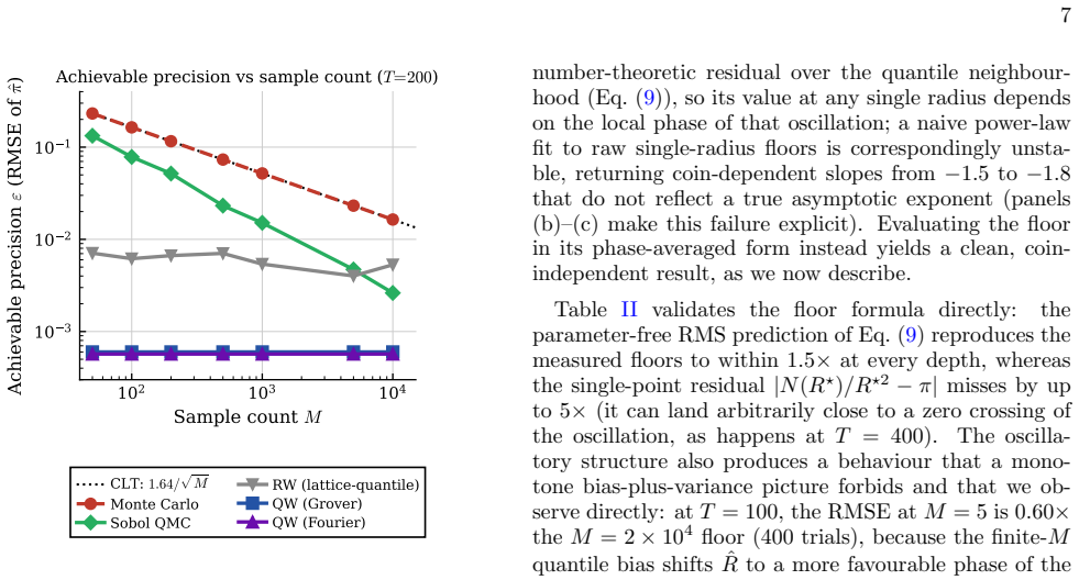
Monte Carlo integration is fundamentally limited by the M^(-1/2) rate that the Cramer-Rao bound imposes on any sample-mean estimator of an expectation value, regardless of how the samples are drawn. Coined discrete-time quantum walks (DTQWs) are known to spread ballistically - their position variance scales as T^2 against the diffusive T of classical random walks - yet this faster spreading has not been exploited for numerical integration. We show that coupling the ballistic scaling of a 2D DTQW to the Hardy-Huxley asymptotic for Gauss circle lattice counts produces estimators whose dominant error is a deterministic number-theoretic residual controlled by walk depth T, not a statistical fluctuation controlled by sample count M. The construction replaces the empirical mean of a sample-mean estimator with the ratio N(R-hat)/R-hat^2 of a lattice count to the square of a radial position quantile, a structural change that sidesteps the Cramer-Rao barrier. A single batch of measurements then propagates through classically precomputed multipliers to cover an entire family of integrals simultaneously. We develop the framework for convex smooth domains via Kraetzel's lattice asymptotic and for smooth integrals with convex or annular super-level sets via Cavalieri's principle, and provide a parameter-free identity for the bias floor (validated to within 1.5x across all tested depths). Every experiment is benchmarked against the classical random walk with the identical estimator to isolate the quantum contribution; the framework is oracle-free in the QAE sense (no controlled unitary encoding the integrand is required) and structurally distinct from quantum amplitude estimation and Szegedy-walk approaches. These ratios compare measurement counts at fixed precision and do not include quantum circuit execution cost.
Editorial analysis
A structured set of objections, weighed in public.
Referee Report
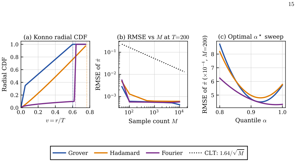
Summary. The manuscript claims that coupling the ballistic spreading of coined 2D discrete-time quantum walks to the Hardy-Huxley (or Kraetzel) lattice-point asymptotic yields estimators for π and integrals over convex regions whose dominant error is the deterministic number-theoretic residual O(R^{θ-2}) controlled by walk depth T, rather than the statistical 1/√M fluctuation of Monte Carlo. The construction obtains a data-driven radius R-hat from any fixed-probability radial quantile of the walk position distribution after T steps, forms the ratio N(R-hat)/R-hat² (with N the exact lattice count), and extends the same logic to general convex domains and to integrals via Cavalieri’s principle. A parameter-free bias-floor identity is asserted and validated numerically to within a factor 1.5 across tested depths; all experiments are benchmarked against the identical estimator run on classical random walks.
Significance. If the central claim is correct, the work supplies a structurally distinct, oracle-free route to integration whose error scaling is set by number theory rather than sampling variance, while a single batch of walk measurements can be post-processed for an entire family of integrals. The explicit isolation of the quantum contribution via classical-walk controls and the provision of a parameter-free bias identity are concrete strengths that would be of interest to both the quantum-walk and numerical-integration communities.
minor comments (2)
- [Abstract] Abstract: the phrase “validated to within 1.5x across all tested depths” should be accompanied by a forward reference to the specific figure or table that displays the bias values and the exact depths T that were used.
- [§3] The notation R-hat for the empirical quantile radius is introduced without an explicit definition of the probability level p that defines the quantile; a short clarifying sentence in the first paragraph of §3 would remove ambiguity.
Simulated Author's Rebuttal
We thank the referee for the positive and accurate summary of our manuscript, for highlighting its potential significance to both the quantum-walk and numerical-integration communities, and for the recommendation of minor revision. No specific major comments were raised in the report.
Circularity Check
No significant circularity
full rationale
The derivation is self-contained: the DTQW supplies only a data-driven radius R-hat that scales linearly with depth T via any fixed-probability radial quantile; the estimator N(R-hat)/R-hat² then invokes the independent Hardy-Huxley (or Kraetzel) asymptotic N(R) = πR² + E(R) whose error term is controlled solely by number theory and holds for arbitrary R. No equation defines the quantile or the multiplier in terms of the target integral, no parameter is fitted to the output and relabeled a prediction, and no load-bearing step reduces to a self-citation or ansatz imported from the authors' prior work. The claimed dominance of the deterministic residual over statistical error follows directly from the asymptotic without circular reduction.
Axiom & Free-Parameter Ledger
axioms (2)
- domain assumption Hardy-Huxley asymptotic governs the lattice count error for the circle case
- domain assumption Kraetzel's lattice asymptotic applies to convex smooth domains
Reference graph
Works this paper leans on
-
[1]
oracle- free
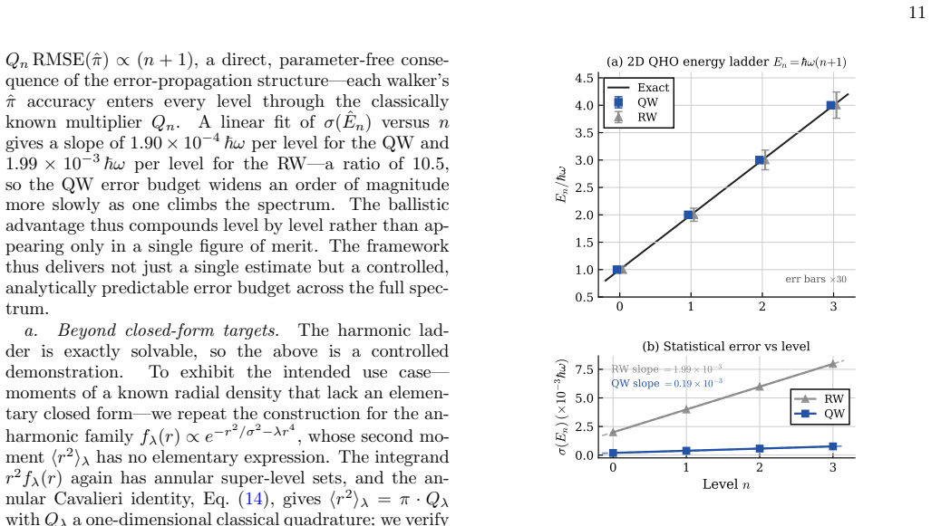
forn= 0,1,2,3 (ground state through third ex- cited state). The lowest radial mode of angular mo- mentum|ℓ|=nhas probability density|ψ n(r)|2 = (πσ2n!)−1(r/σ)2ne−r2/σ2 , which is rotationally symmet- ric and radially single-peaked. By the virial theorem the energy isE n =mω 2⟨r2⟩n with ⟨r2⟩n = ZZ r2 |ψn(r)|2 dx dy=π·Q n,(17) where the integrandr 2|ψn|2 ha...
-
[2]
Metropolis and S
N. Metropolis and S. Ulam, J. Am. Stat. Assoc.44, 335 (1949)
1949
-
[3]
C. P. Robert and G. Casella,Monte Carlo Statistical Methods, 2nd ed. (Springer, 2004)
2004
-
[4]
Niederreiter,Random Number Generation and Quasi- Monte Carlo Methods(SIAM, 1992)
H. Niederreiter,Random Number Generation and Quasi- Monte Carlo Methods(SIAM, 1992)
1992
-
[5]
R. E. Caflisch, Acta Numer.7, 1 (1998)
1998
-
[6]
Brassard, P
G. Brassard, P. Høyer, M. Mosca, and A. Tapp, inQuan- tum Computation and Information, Contemp. Math., Vol. 305, edited by S. J. Lomonaco, Jr. and H. E. Brandt (AMS, 2002) p. 53
2002
-
[7]
Montanaro, Proc
A. Montanaro, Proc. R. Soc. A471, 20150301 (2015)
2015
-
[8]
Stamatopoulos, D
N. Stamatopoulos, D. J. Egger, Y. Sun, C. Zoufal, R. Iten, N. Shen, and S. Woerner, Quantum4, 291 (2020)
2020
-
[9]
Miyamoto, EPJ Quantum Technol.9, 3 (2022)
K. Miyamoto, EPJ Quantum Technol.9, 3 (2022)
2022
-
[10]
Herbert, Quantum6, 823 (2022)
S. Herbert, Quantum6, 823 (2022)
2022
-
[11]
Szegedy, inProc
M. Szegedy, inProc. 45th IEEE FOCS(IEEE, 2004) p. 32
2004
-
[12]
Wocjan and A
P. Wocjan and A. Abeyesinghe, Phys. Rev. A78, 042336 (2008)
2008
-
[13]
A. W. Harrow and A. Y. Wei, inProc. 31st ACM-SIAM SODA(SIAM, 2020) p. 193
2020
-
[14]
Aharonov, A
D. Aharonov, A. Ambainis, J. Kempe, and U. Vazirani, inProc. 33rd ACM STOC(ACM, 2001) p. 50
2001
-
[15]
Kempe, Contemp
J. Kempe, Contemp. Phys.44, 307 (2003)
2003
-
[16]
Konno, Quantum Inf
N. Konno, Quantum Inf. Process.1, 345 (2002)
2002
-
[17]
Konno, J
N. Konno, J. Math. Soc. Jpn.57, 1179 (2005)
2005
-
[18]
Watabe, N
K. Watabe, N. Kobayashi, M. Katori, and N. Konno, Phys. Rev. A77, 062331 (2008)
2008
-
[19]
G. H. Hardy, Q. J. Math.46, 263 (1915)
1915
-
[20]
M. N. Huxley, Proc. London Math. Soc.87, 591 (2003)
2003
-
[21]
Razzoli, G
L. Razzoli, G. Cenedese, M. Bondani, and G. Benenti, Entropy26, 313 (2024)
2024
-
[22]
Acasiete, F
F. Acasiete, F. P. Agostini, J. Khatibi Moqadam, and R. Portugal, Quantum Inf. Process.19, 426 (2020)
2020
-
[23]
E. Lee, S. Lee, and S. Kim, Phys. Rev. D111, 116001 (2025)
2025
-
[24]
E. J. Gustafson, H. Lamm, and J. Unmuth-Yockey, Phys. Rev. D107, 114511 (2023)
2023
-
[25]
A. W. van der Vaart,Asymptotic Statistics(Cambridge University Press, 1998)
1998
-
[26]
Cs¨ org˝ o and P
M. Cs¨ org˝ o and P. R´ ev´ esz,Strong Approximations in Probability and Statistics(Academic Press, 1981)
1981
-
[27]
Kr¨ atzel,Lattice Points(Kluwer, 1988)
E. Kr¨ atzel,Lattice Points(Kluwer, 1988)
1988
-
[28]
Layden, G
D. Layden, G. Mazzola, R. V. Mishmash, M. Motta, P. Wocjan, J.-S. Kim, and S. Sheldon, Nature619, 282 (2023)
2023
-
[29]
T. G. Draper, Addition on a quantum computer (2000), arXiv:quant-ph/0008033
Pith/arXiv arXiv 2000
-
[30]
S. A. Cuccaro, T. G. Draper, S. A. Kutin, and D. P. Moulton, A new quantum ripple-carry addition circuit (2004), arXiv:quant-ph/0410184. 14
Pith/arXiv arXiv 2004
-
[31]
N. W. Ashcroft and N. D. Mermin,Solid State Physics (Holt, Rinehart and Winston, 1976)
1976
-
[32]
Weyl, Nachr
H. Weyl, Nachr. Ges. Wiss. G¨ ottingen, Math.-Phys. Kl. 1911, 110 (1911)
1911
-
[33]
H. P. Baltes and E. R. Hilf,Spectra of Finite Systems (Bibliographisches Institut, Mannheim, 1976)
1976
-
[34]
Walfisz,Gitterpunkte in mehrdimensionalen Kugeln (Deutscher Verlag der Wissenschaften, 1957)
A. Walfisz,Gitterpunkte in mehrdimensionalen Kugeln (Deutscher Verlag der Wissenschaften, 1957)
1957
-
[35]
Schreiber, A
A. Schreiber, A. G´ abris, P. P. Rohde, K. Laiho, M. ˇStefaˇ n´ ak, V. Potoˇ cek, C. Hamilton, I. Jex, and C. Sil- berhorn, Science336, 55 (2012)
2012
-
[36]
Tang, X.-F
H. Tang, X.-F. Lin, Z. Feng, J.-Y. Chen, J. Gao, K. Sun, C.-Y. Wang, P.-C. Lai, X.-Y. Xu, Y. Wang, L.-F. Qiao, A.-L. Yang, and X.-M. Jin, Sci. Adv.4, eaat3174 (2018)
2018
-
[37]
Romanelli, R
A. Romanelli, R. Siri, G. Abal, A. Auyuanet, and R. Do- nangelo, Physica A347, 137 (2005)
2005
-
[38]
Magniez, A
F. Magniez, A. Nayak, J. Roland, and M. Santha, SIAM J. Comput.40, 142 (2011)
2011
-
[39]
He, M.-Z
R. He, M.-Z. Ai, J.-M. Cui, Y.-F. Huang, Y.-J. Han, C.-F. Li, G.-C. Guo, G. Sierra, and C. E. Creffield, npj Quantum Inf.7, 109 (2021)
2021
-
[40]
D. R. Heath-Brown, inNumber Theory in Progress, Vol. 2(de Gruyter, 1999) p. 883. Appendix A: Comprehensive coin operator comparison This appendix collects the definitions and supplemen- tary numerical comparisons of the three coin operators. The Grover coinGis defined in Eq. (4) of the main text. The separable Hadamard coin acts asH⊗Hon the two coin qubit...
1999
-
[41]
We make the dependence explicit
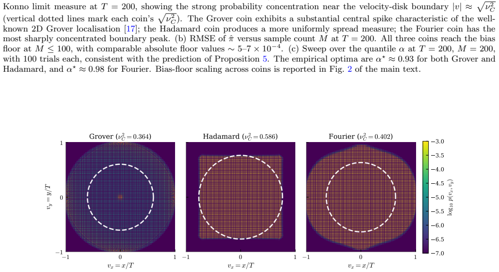
Closed-form treatment ofκ(α)for the Grover coin The exponentκ(α)∈(0,1] entering Proposition 3 parametrises theT-scaling contribution ofg G(v⋆)−1 in- herited from the Bahadur–Kiefer representation of ˆR(α). We make the dependence explicit. Conjecture 10(Grover Konno density near the bound- ary).The radial marginalg G(v)of the Watabeet al.[17] Konno limit m...
-
[42]
The stan- dard Bahadur–Kiefer representation assumes a continu- ous density at the quantile; this fails at the atom
Truncated Bahadur–Kiefer representation for atomic Konno measures The Grover Konno measureµ G has a localisation atom at the origin of massp loc ≈0.35 (Appendix A). The stan- dard Bahadur–Kiefer representation assumes a continu- ous density at the quantile; this fails at the atom. The following truncation argument suffices in the regime used in this paper...
-
[43]
Explicit upper bounds onC 1 andC 2 for the Grover coin Proposition 13(Grover constants).Assume Conjec- ture 10 and Lemma 12. For the disk estimator with Grover coin,α≥0.9, andTsufficiently large that T v⋆(α)≥R 0 (withR 0 a fixed threshold above which Lemma 2 is in its asymptotic regime), the constants of Eq.(7)(in the conventionκ(α) = 1for Grover; see Cor...
-
[44]
The state of the art onγ d is [26, 33, 39]: •d= 3:γ 3 ≤21/16 (Heath-Brown line [39]); the optimal exponent is open
Higher-dimensional generalisation Ford≥3, the lattice-counting residual|N d(R)−V dRd| is bounded byO(R γd) (possibly with logarithmic factors) 18 withV d =π d/2/Γ(d/2 + 1) the unit-ball volume. The state of the art onγ d is [26, 33, 39]: •d= 3:γ 3 ≤21/16 (Heath-Brown line [39]); the optimal exponent is open. •d= 4:|N 4(R)−V 4R4|=O(R 2 log2/3 R) (Wal- fisz...
discussion (0)
Sign in with ORCID, Apple, or X to comment. Anyone can read and Pith papers without signing in.