A hybrid method for reconstruction of the equation of state of dark energy and its application to Pantheon+SH0ES data
Pith reviewed 2026-06-25 21:32 UTC · model grok-4.3
The pith
A hybrid reconstruction derives the dark energy equation of state from distance data and finds consistency with w = -1.
A machine-rendered reading of the paper's core claim, the machinery that carries it, and where it could break.
Core claim
By reconstructing the equation of state from the dimensionless comoving distance D(z) and its derivatives instead of imposing a predefined parametric form on w(z), the hybrid method applied to Pantheon+ SH0ES data produces a reconstruction consistent with dark energy as a cosmological constant where w equals -1.
What carries the argument
The hybrid semi-parametric reconstruction that parametrizes the distance-redshift relation D(z) and extracts w(z) from its first and second derivatives.
If this is right
- Dark energy constraints can be derived without first choosing a specific functional form for w(z).
- The Pantheon+ SH0ES data do not require a dynamical dark energy component beyond the cosmological constant.
- Future surveys that increase the number of distance measurements will produce tighter bounds on any possible deviation of w from -1.
Where Pith is reading between the lines
- The same derivative-based extraction could be applied to combined datasets that include baryon acoustic oscillation measurements to test consistency across probes.
- If larger samples later show w departing from -1 at higher redshifts, the reconstruction would naturally favor models in which dark energy evolves with time.
- The approach supplies a route to model-independent checks that might help address current tensions among cosmological parameter estimates.
Load-bearing premise
The method still requires adopting functional representations for the distance-redshift relation itself.
What would settle it
A statistically significant deviation of the reconstructed w(z) from -1 when the same method is applied to a substantially larger supernova sample from a future survey such as LSST would falsify the consistency result.
Figures
read the original abstract
Cosmology aims to understand the physical properties of our Universe on its largest scales. One such feature is the expansion of the Universe, which currently seems to be dominated by a phenomenon referred to as dark energy. The physical nature and properties of dark energy are one of the main topics of investigation of modern cosmology. Observational cosmology aims to reconstruct the evolution and the equation of state of dark energy, while theoretical cosmology aims to provide methods for such reconstructions and models explaining the nature of dark energy. If the equation of state, defined as the ratio of pressure to density $w = p/\rho$, deviates from $-1$, i.e. $w\ne-1$, then this would imply the existence of some sort of dynamical process behind dark energy. Most investigations assume a specific parametric form of $w$, eg. $w(z) = w_{0} + w_a z/(1+z)$, with $z$ being redshift and $w_0$ and $w_a$ being constants. The analysis of the data is then reduced to fitting the model to the data. In this work, we take a different approach. Instead of imposing a predefined parametric form for $w(z)$, we reconstruct the equation of state indirectly from the dimensionless comoving distance $D(z)$ and its derivatives. This avoids assuming a specific physical parametrisation of dark energy, such as the CPL form, but still requires adopting functional representations for the distance--redshift relation itself. The method should therefore be regarded as a hybrid or semi-parametric reconstruction approach: the parametrisation is shifted from the equation of state to the observable distance function. Finally we apply the method to the Pantheon+ SH0ES data. The results are consistent with dark energy being the cosmological constant, i.e. $w = -1$. Future surveys such as LSST will provide more data and narrow down the uncertainty. This in turn will yield tighter constraints on dark energy.
Editorial analysis
A structured set of objections, weighed in public.
Referee Report
Summary. The paper proposes a hybrid reconstruction method for the dark energy equation of state w(z) that derives it from the dimensionless comoving distance D(z) and its first and second derivatives rather than assuming a parametric form such as CPL for w(z) itself. The approach is applied to the Pantheon+SH0ES supernova dataset and yields results consistent with a cosmological constant (w = -1). The abstract notes that a functional representation for D(z) must still be adopted.
Significance. If the reconstruction proves robust to the choice of basis or knot placement for D(z) and includes explicit error propagation and cross-checks, the method would offer a useful semi-parametric alternative to fully parametric w(z) fits, allowing data-driven tests for dynamical dark energy while shifting the modeling assumptions to the observable distance-redshift relation. The reported consistency with w = -1 would then provide supporting evidence for LambdaCDM from this particular reconstruction route.
major comments (2)
- [Abstract] Abstract: the central claim that the results are consistent with w = -1 cannot be evaluated because the text supplies no information on the specific functional forms adopted for D(z), the number or placement of free parameters in that representation, the propagation of uncertainties through the second derivative, or any robustness tests against alternative bases. This is load-bearing for the conclusion, as the skeptic note correctly identifies that an insufficiently flexible D(z) representation can suppress detectable deviations from w = -1 after differentiation.
- [Abstract] The hybrid character of the method (explicitly acknowledged in the abstract) means that the derived w(z) is not parameter-free; any fitted parameters in the D(z) representation enter the final result by construction. Without a quantitative demonstration that the chosen representation is flexible enough to recover injected dynamical signals at the level of the Pantheon+SH0ES errors, the consistency with w = -1 remains conditional on modeling choices whose impact is not quantified.
minor comments (1)
- [Abstract] The abstract would benefit from a brief statement of the concrete functional form(s) ultimately used for D(z) and the number of free parameters involved.
Simulated Author's Rebuttal
We thank the referee for the careful and constructive review. The comments correctly identify that the abstract is too concise to allow independent evaluation of the central claim and that the hybrid character of the method requires explicit justification of the D(z) representation's flexibility. We address both points below and will revise the manuscript accordingly.
read point-by-point responses
-
Referee: [Abstract] Abstract: the central claim that the results are consistent with w = -1 cannot be evaluated because the text supplies no information on the specific functional forms adopted for D(z), the number or placement of free parameters in that representation, the propagation of uncertainties through the second derivative, or any robustness tests against alternative bases. This is load-bearing for the conclusion, as the skeptic note correctly identifies that an insufficiently flexible D(z) representation can suppress detectable deviations from w = -1 after differentiation.
Authors: We agree that the abstract, in its current form, does not supply these details and therefore does not permit the reader to assess the claim independently. The main text (Section 3) specifies the functional representation adopted for D(z), the number and placement of parameters, the Monte-Carlo procedure used to propagate uncertainties through the second derivative, and the robustness checks against alternative bases. To remedy the deficiency noted by the referee we will expand the abstract with a concise statement that (i) identifies the representation and parameter count, (ii) notes that uncertainties are propagated via sampling, and (iii) states that the reported consistency with w = -1 is stable under the robustness tests described in the body of the paper. revision: yes
-
Referee: [Abstract] The hybrid character of the method (explicitly acknowledged in the abstract) means that the derived w(z) is not parameter-free; any fitted parameters in the D(z) representation enter the final result by construction. Without a quantitative demonstration that the chosen representation is flexible enough to recover injected dynamical signals at the level of the Pantheon+SH0ES errors, the consistency with w = -1 remains conditional on modeling choices whose impact is not quantified.
Authors: We accept the referee's observation that the hybrid construction makes the final w(z) dependent on the flexibility of the D(z) representation. The manuscript already contains comparisons with parametric models and limited simulated-data checks (Section 5) that indicate the chosen representation can accommodate deviations from w = -1. Nevertheless, these checks fall short of the explicit, quantitative injection-recovery test at the Pantheon+SH0ES error level that the referee requests. We will therefore add such a test in the revised manuscript, reporting recovery statistics for injected dynamical signals of amplitude comparable to the current data uncertainties. This addition will make the conditional nature of the result explicit and will quantify the impact of the modeling choices. revision: yes
Circularity Check
No significant circularity; hybrid reconstruction is data-driven
full rationale
The paper explicitly describes its approach as hybrid/semi-parametric, shifting parametrization from w(z) to a chosen functional form for D(z) while reconstructing w from D(z) and derivatives. This is applied to Pantheon+SH0ES data to obtain consistency with w=-1. No quoted step shows a result equivalent to its inputs by construction, no fitted parameter renamed as prediction, and no load-bearing self-citation or uniqueness theorem. The derivation chain from observed distances to w(z) follows standard cosmological relations and remains independent of the final claim.
Axiom & Free-Parameter Ledger
free parameters (1)
- parameters defining the functional form of D(z)
axioms (1)
- domain assumption Standard FLRW metric relations that connect the comoving distance and its derivatives to the equation of state w(z)
Reference graph
Works this paper leans on
-
[1]
Introducing the dimensionless comoving distance D as D(z) = H0 c d(z), (4) and assuming spatial flatness, eq
for w. Introducing the dimensionless comoving distance D as D(z) = H0 c d(z), (4) and assuming spatial flatness, eq. ( 1) can be rearranged to (cf. Appendix A) [10]. w = 2 3 D′′ D′ (1 + z) + 1 Ω M (1 + z)3D′2 − 1 . (5) This reformulation has an important implication. In the standard approach, the dependence of observables on w(z) enters through multiple in...
-
[2]
This has the potential to re- veal time variation in w(z) that may otherwise be hidden by the integrated nature of distance measurements
expresses w(z) in terms of derivatives of the distance- redshift relation, making the reconstruction sensitive to local structure in the data. This has the potential to re- veal time variation in w(z) that may otherwise be hidden by the integrated nature of distance measurements. Despite this advantage, the direct application of eq. ( 5) presents several ...
-
[3]
A further challenge of this approach is the numerical instability inherent in estimating derivatives from noisy data
still requires knowledge about Ω M and H0. A further challenge of this approach is the numerical instability inherent in estimating derivatives from noisy data. The reconstruction of w(z) depends explicitly on both D′(z) and D′′(z), making it sensitive to small-scale fluctuations in the inferred distance–redshift relation. In the presence of noise, direct ...
-
[4]
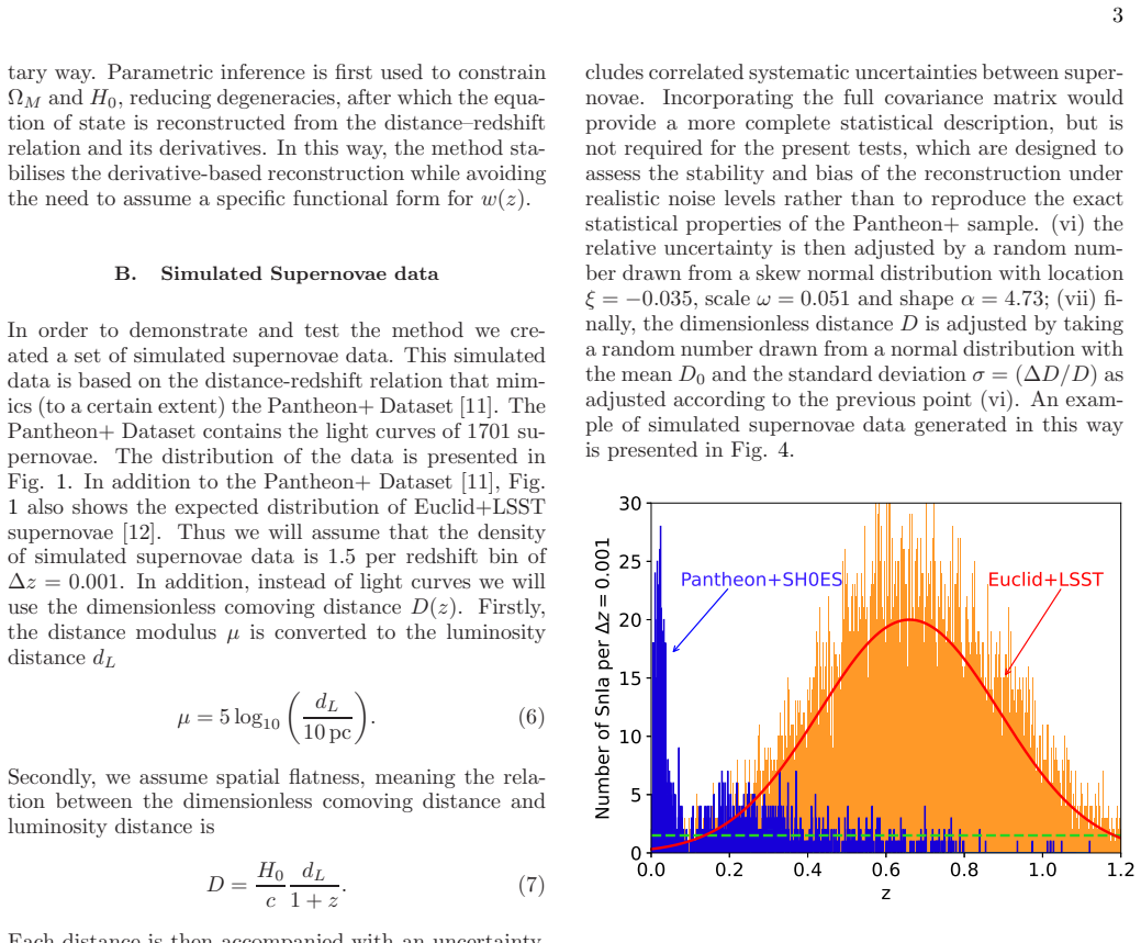
1 also shows the expected distribution of Euclid+LSST supernovae [12]
In addition to the Pantheon+ Dataset [11], Fig. 1 also shows the expected distribution of Euclid+LSST supernovae [12]. Thus we will assume that the density of simulated supernovae data is 1.5 per redshift bin of ∆ z = 0 . 001. In addition, instead of light curves we will use the dimensionless comoving distance D(z). Firstly, the distance modulus µ is conv...
-
[5]
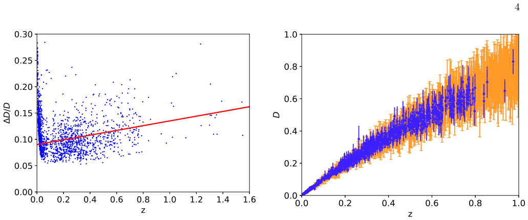
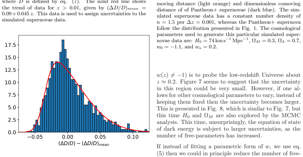
09 + 0. 045 z. This data is used to assign uncertainties to the simulated supernovae data. −0.05 0.00 0.05 0.10 (/uni0394 D / D Δ − (/uni0394 D / D Δ mean 0.0 2.5 5.0 7.5 10.0 12.5 15.0 17.5 FIG. 3. The distribution of residuals of relative uncertain ties: ∆ D/D − (∆ D/D )mean, cf. Fig. 1. The solid red curve is the skew normal distribution with the follo...
-
[6]
This however is more difficult to implement than it initially sounds
then we could in principle reduce the number of free- parameters and consequently keep the uncertainties un- der control. This however is more difficult to implement than it initially sounds. First we do require the deriva- tives of D. Given large uncertainties in the data we try to overcome this by fitting a polynomial to the distance data instead. As a firs...
-
[7]
To overcome this hurdle we use the MCMC chains for Ω M and H0 from the previous method
requires knowledge of Ω M and H0. To overcome this hurdle we use the MCMC chains for Ω M and H0 from the previous method. The outcome is presented in Fig. 9. While the uncertainties and sensitivity to reconstruct w(z) is not diametrically different than the standard MCMC methods, it provides a different way of inferring the equation of state, and thus promp...
-
[8]
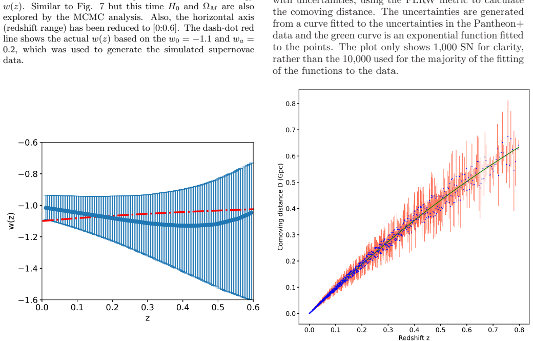
are derivatives of D. By fitting a smooth function to the comoving dis- tance data, and taking its first and second derivatives, it is possible to retrieve the equation of state of dark energy w from the data. Uncertainties in w can also be calcu- lated by propagating the covariance matrix of any fitted function through the derivatives of the function, plus ...
-
[9]
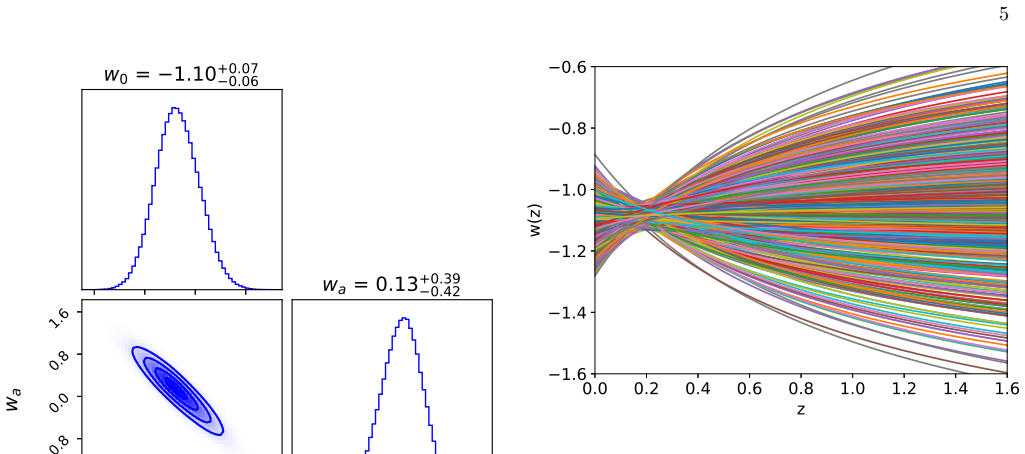
0.0 0.1 0.2 0.3 0.4 0.5 0.6 z −1.6 −1.4 −1.2 −1.0 −0.8 −0.6 w(z) FIG
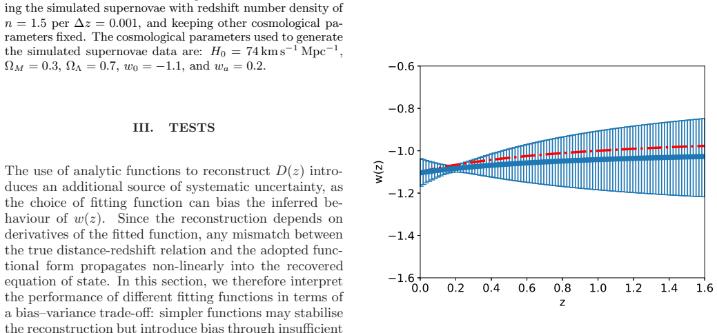
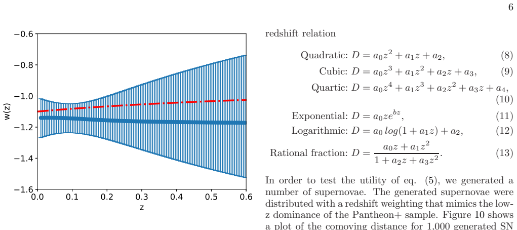
2, which was used to generate the simulated supernovae data. 0.0 0.1 0.2 0.3 0.4 0.5 0.6 z −1.6 −1.4 −1.2 −1.0 −0.8 −0.6 w(z) FIG. 9. Reconstruction of the equation of state of dark energ y w(z). Similar to Fig. 8 but the equation of state was inferred using eq. (5). The dash-dot red line shows the actual w(z) based on the w0 = − 1. 1 and wa = 0 . 2, whic...
-
[10]
The different quantities of SN generated were to determine how many were necessary to recover w effectively
to attempt to recover w. The different quantities of SN generated were to determine how many were necessary to recover w effectively. The parame- ters used to generate the simulated supernovae data were H0 = 73. 30± 1. 04 km s − 1 Mpc− 1 [5], Ω M = 0. 334± 0. 018
-
[11]
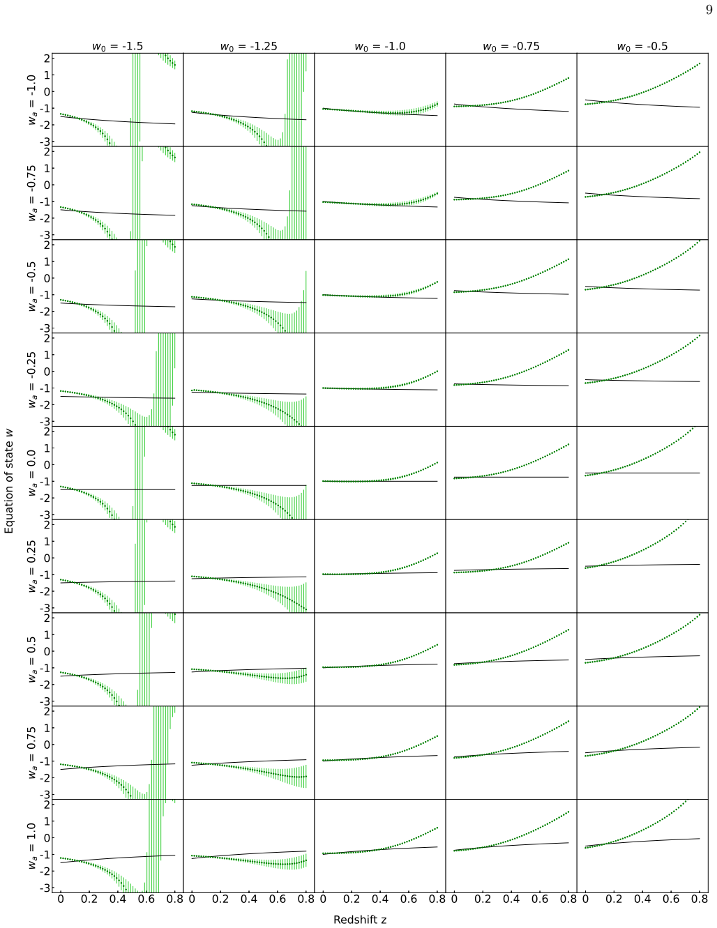
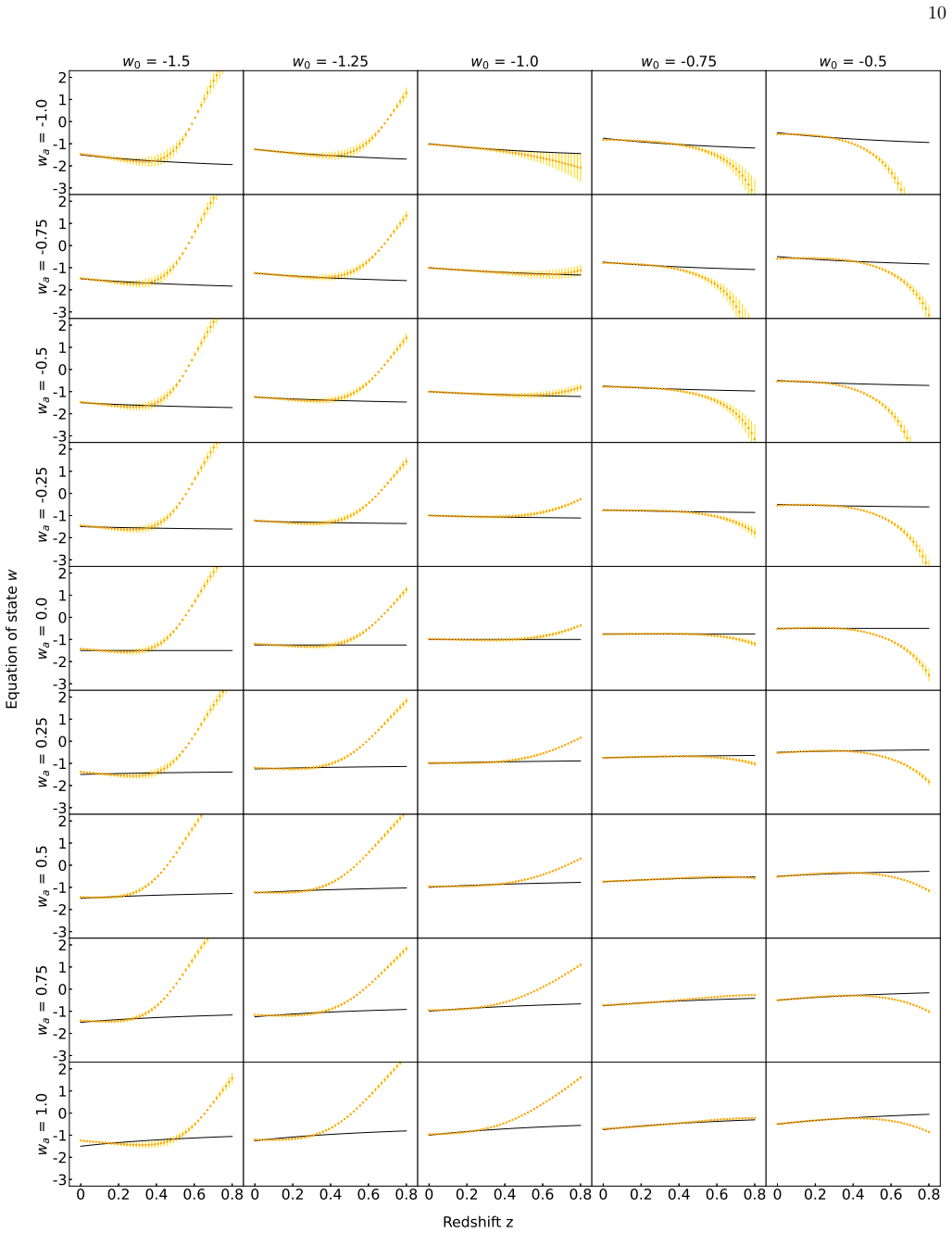
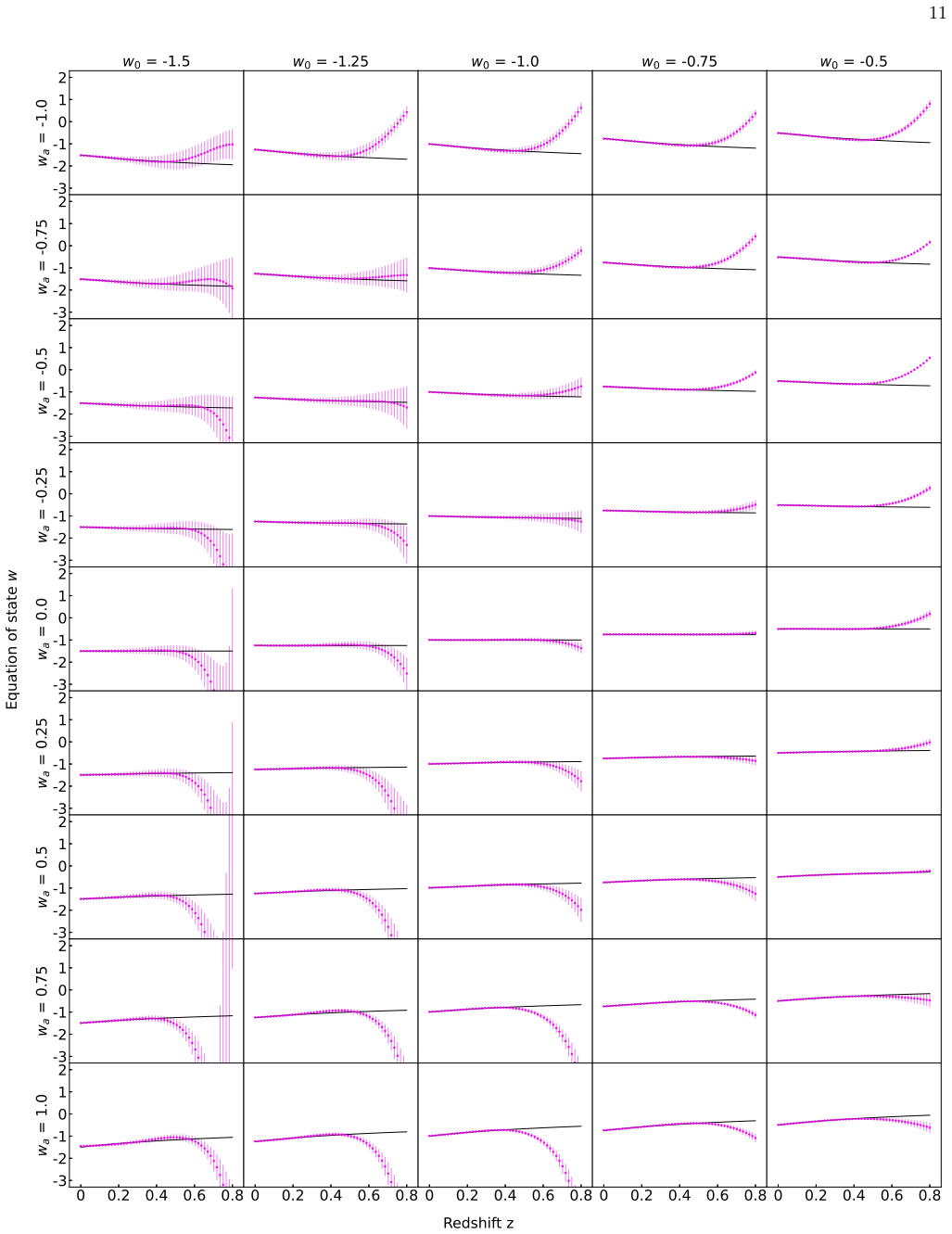
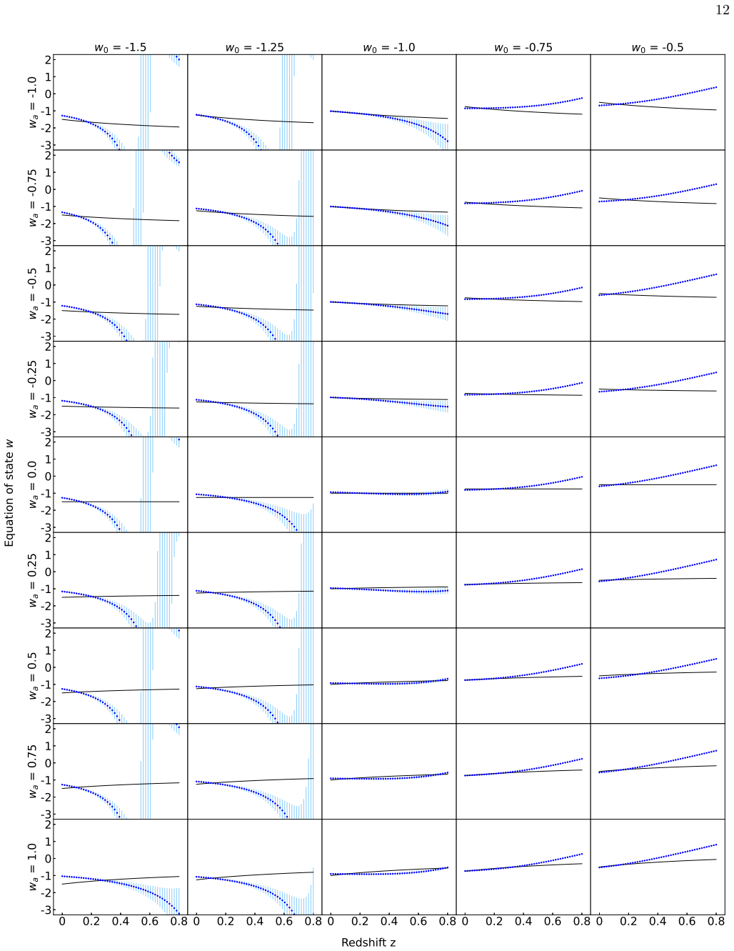
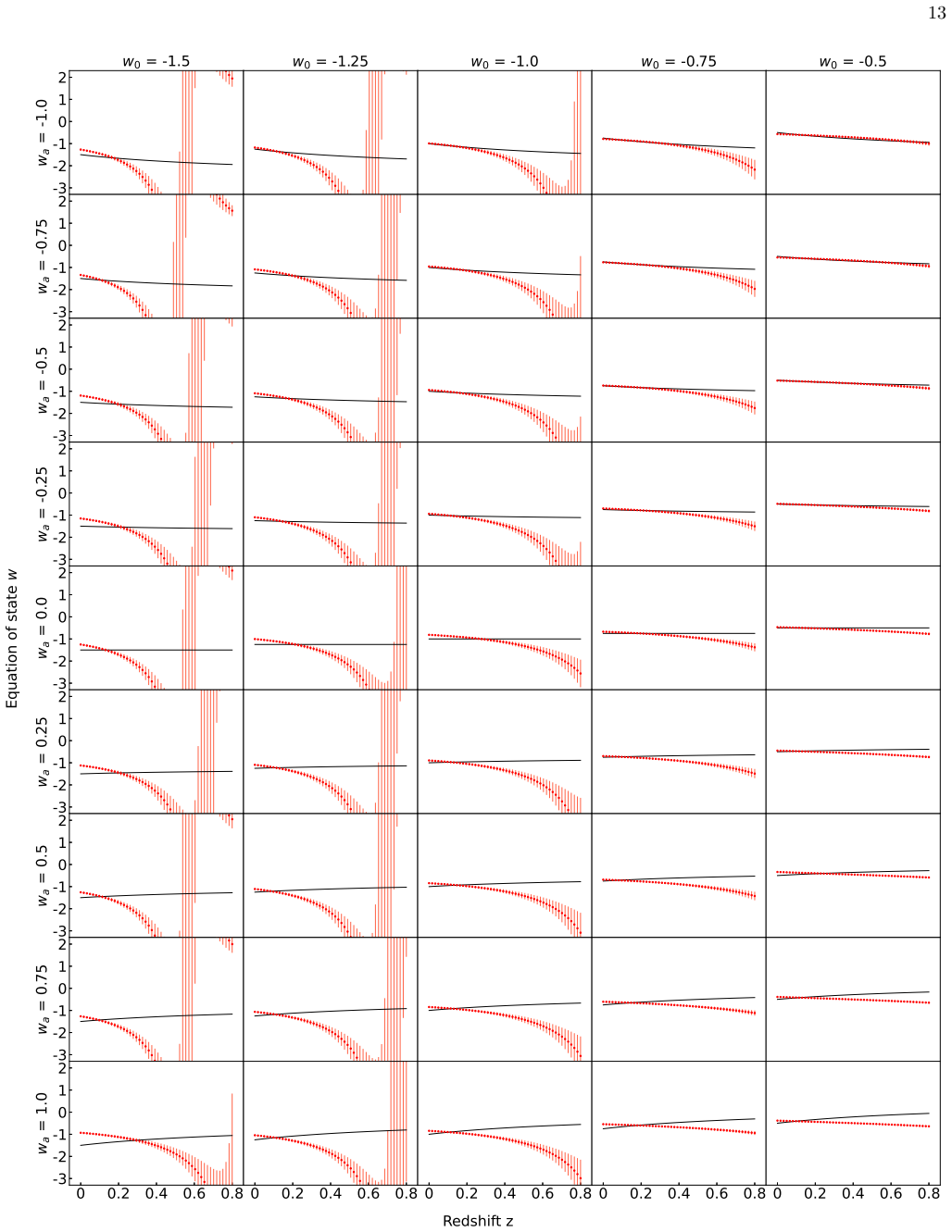
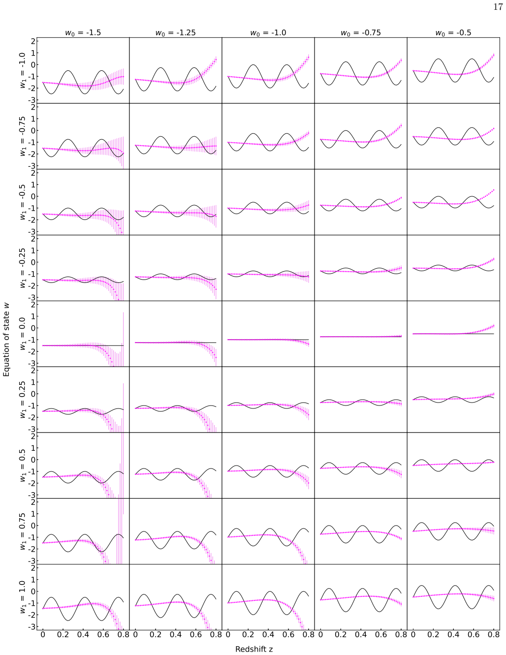
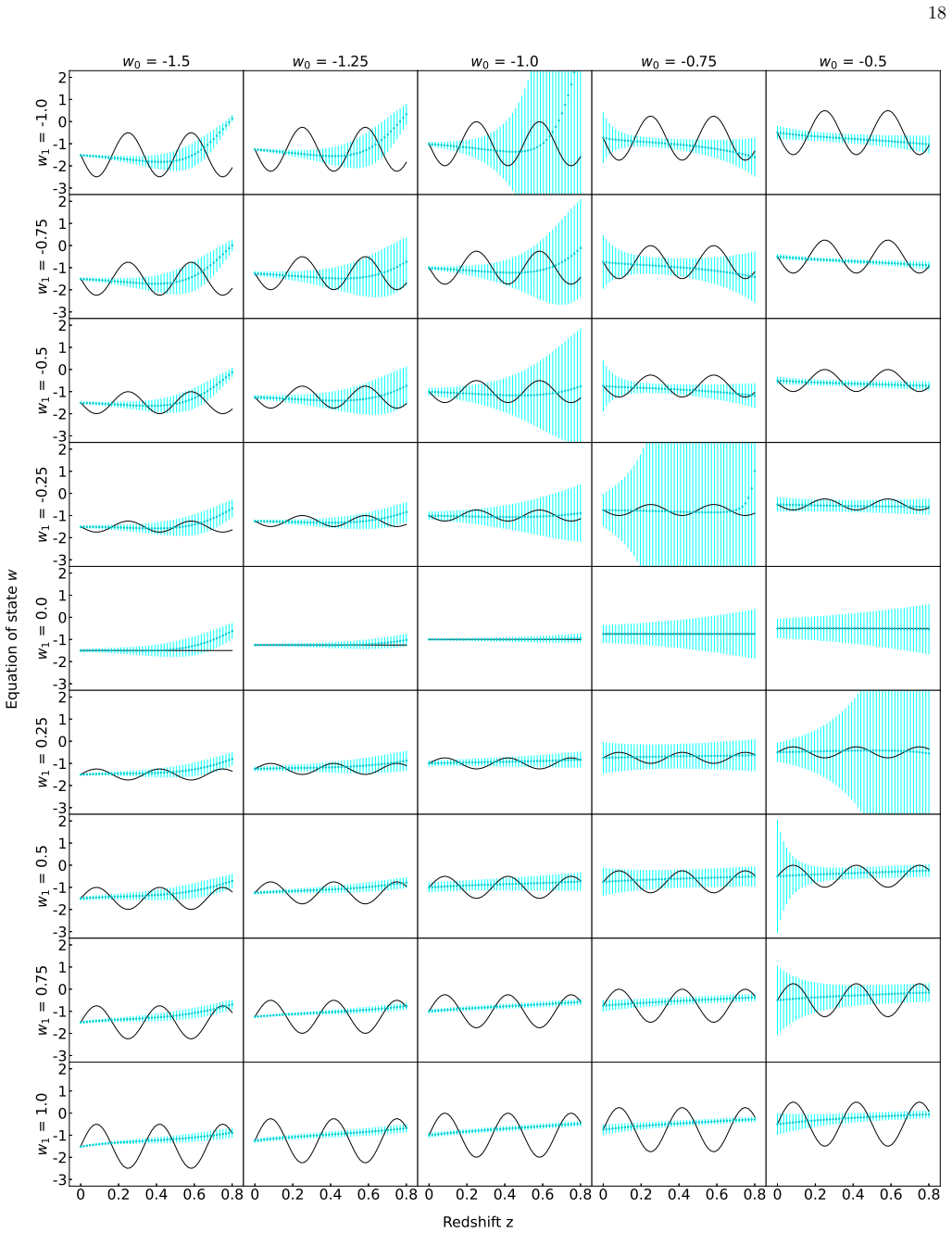
Figures 12 to 17 in show the derived equation of state w for curves fitted to 10,000 generated Supernovae for redshift z from 0 to 0.8
and Ω Λ = 1 − Ω M . Figures 12 to 17 in show the derived equation of state w for curves fitted to 10,000 generated Supernovae for redshift z from 0 to 0.8. The curves fitted to the data are quadratic, cubic, quartic, exponential, logarithmic and rational fraction, respectively. Each shows the equation of state w obtained from fitting the curve and applying e...
-
[12]
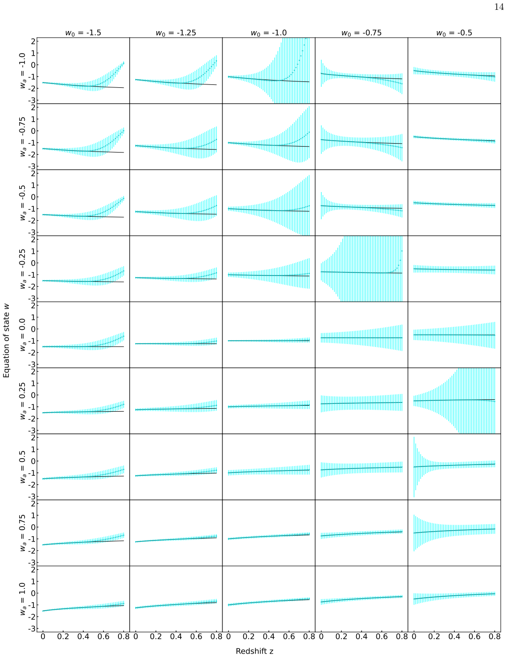
4; for other values it fails to reproduce the under- lying behaviour
recov- ers w accurately only when w0 = − 1 and only up to z = 0 . 4; for other values it fails to reproduce the under- lying behaviour. Similarly, the cubic (Fig. 13) provides a slightly better reconstruction but only up to z = 0 . 4 in most cases. Only for a very few combinations of w0 and wa is there a good fit up to z = 0 . 8, such as for w0 = − 1, w a ...
-
[13]
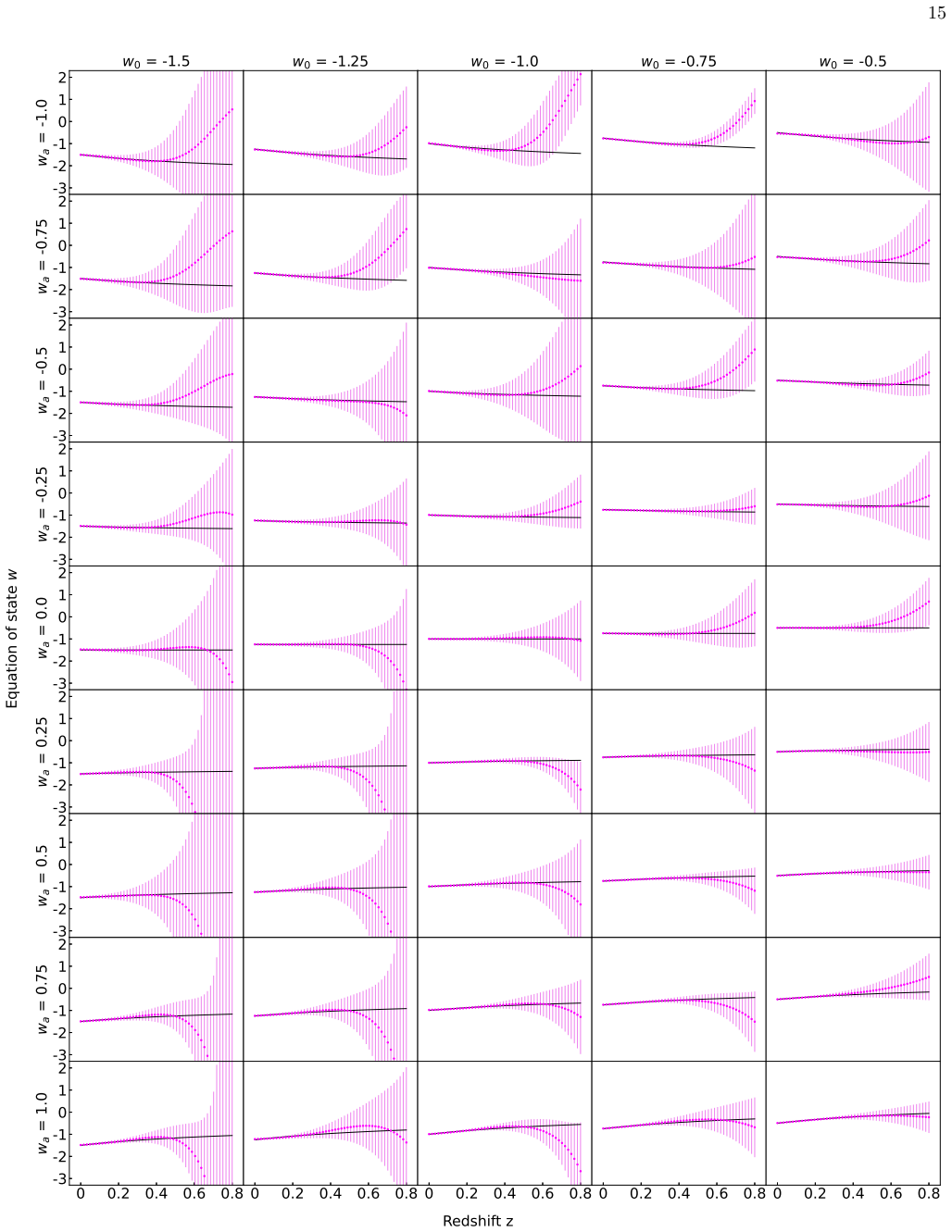
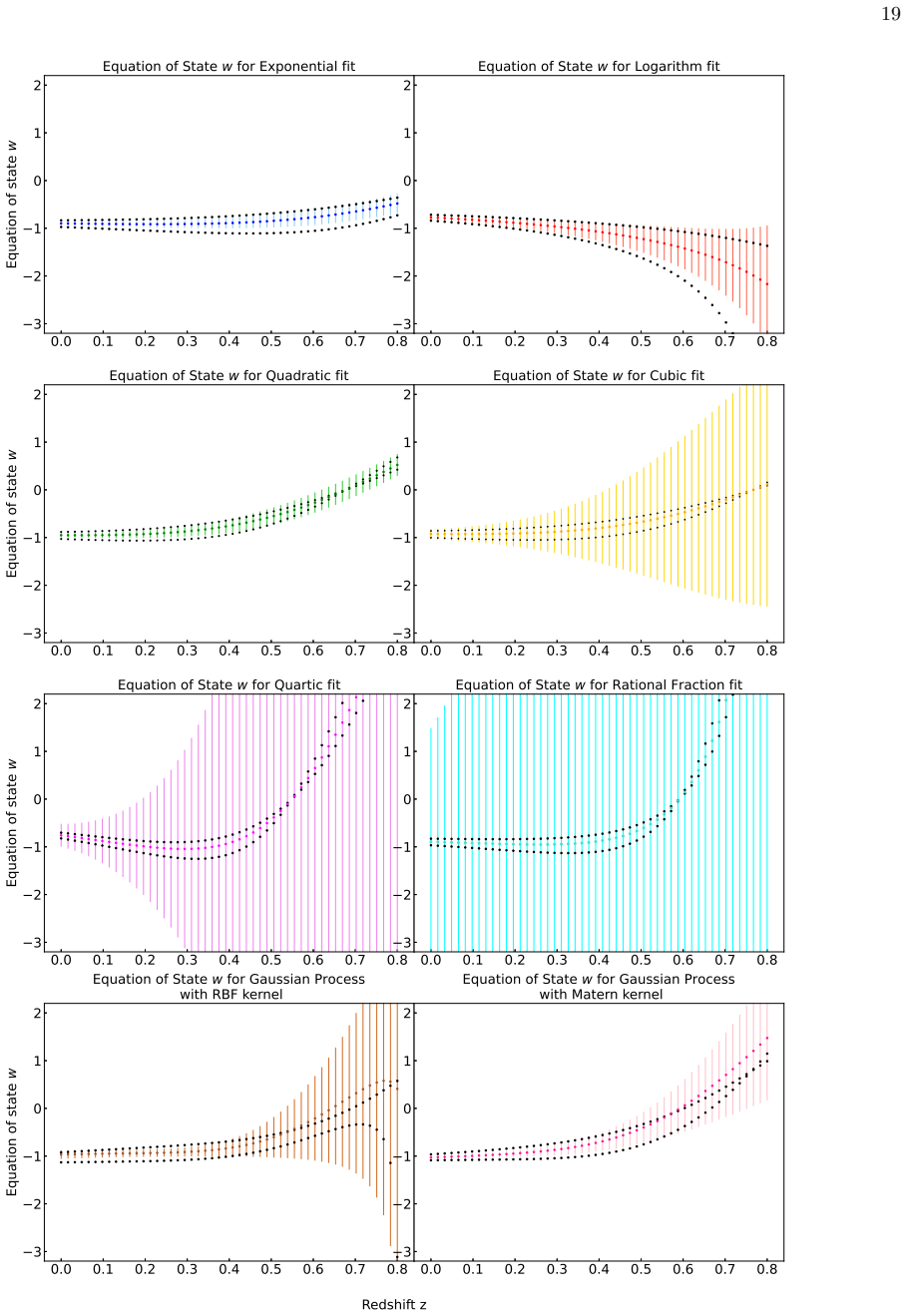
16) fits generally provide poor recon- structions of w(z)
and logarithmic (Fig. 16) fits generally provide poor recon- structions of w(z). The exponential fit performs well only in limited cases where w0 = − 1, while the logarithmic form provides a reasonable fit only for a small subset of models, typically where w0 = − 0. 75 or − 0. 5 and wa < 0, and therefore neither are robust reconstruction methods. The rationa...
-
[14]
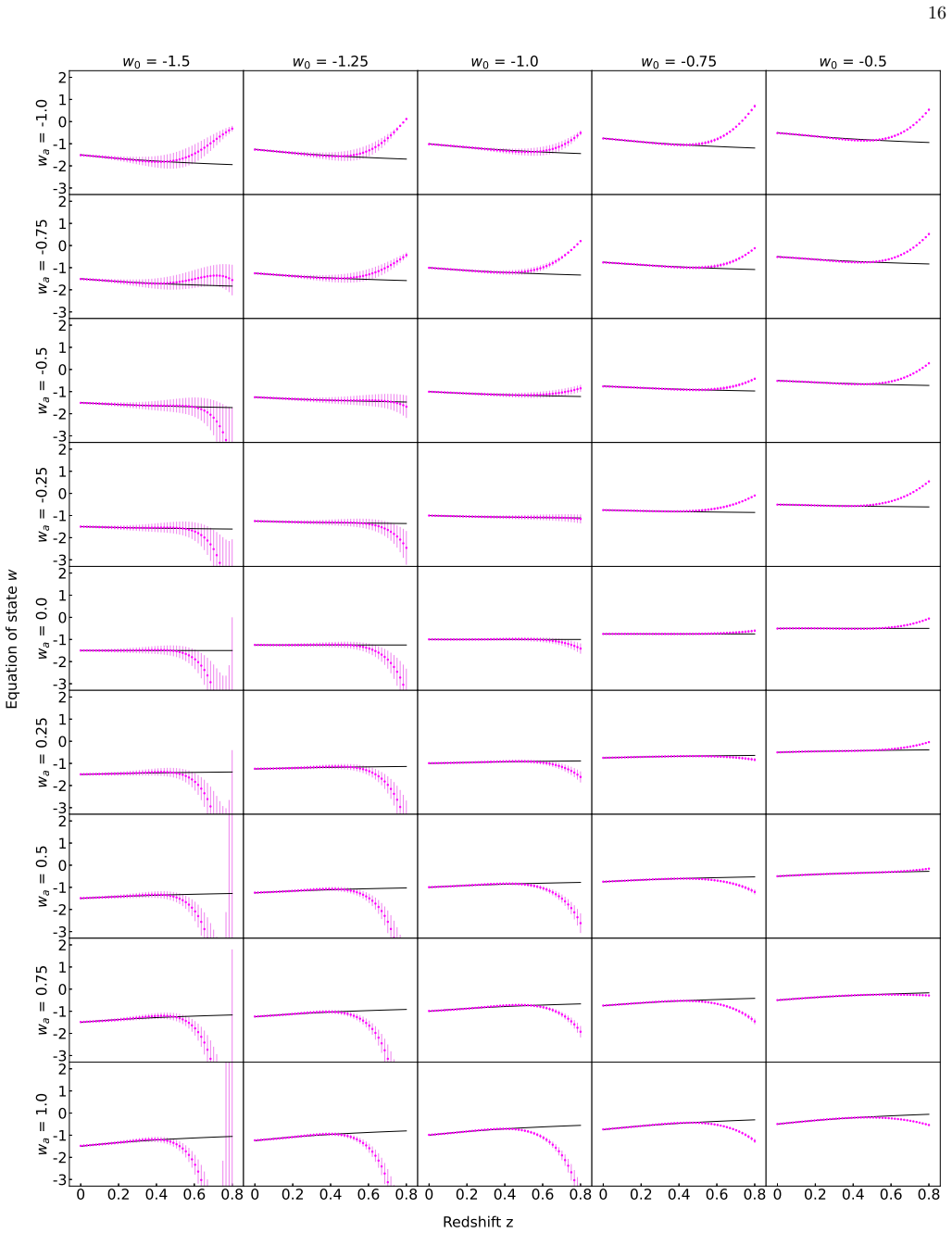
8 in most cases, but with larger un- certainties than other fits
provides the most accu- rate recovery of w across the range of w0 and wa, fitting well up to z = 0 . 8 in most cases, but with larger un- certainties than other fits. The larger uncertainties are due to the more complicated rational fraction equation allowing more freedom when fitted to the data. The ra- tional fraction is also a likely candidate for applyin...
-
[15]
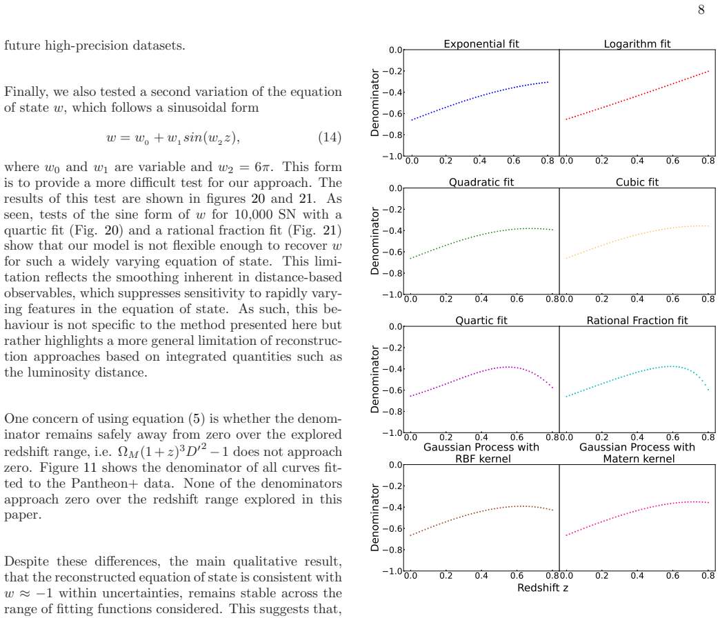
Ω M (1 +z)3D′2 − 1 does not approach zero
is whether the denom- inator remains safely away from zero over the explored redshift range, i.e. Ω M (1 +z)3D′2 − 1 does not approach zero. Figure 11 shows the denominator of all curves fit- ted to the Pantheon+ data. None of the denominators approach zero over the redshift range explored in this paper. Despite these differences, the main qualitative resul...
-
[16]
The black curve represents w from the CPL equation (eq
from -1.5 to -0.5 horizontally, and -1 to 1 vertically, bot h with a step of 0.25. The black curve represents w from the CPL equation (eq. 3) for the same values. The parameters used to g enerate the simulated SN were the same as for Fig. 12. 11 2 1 0 -1 -2 -3 w a = -1.0 w 0 = -1.5 w 0 = -1. 25 w 0 = -1.0 w 0 = -0. 75 w 0 = -0.5 2 1 0 -1 -2 -3 w a = -0. 7...
-
[17]
The black curve represents w from the CPL equation (eq
from -1.5 to -0.5 horizontally, and -1 to 1 vertically, bot h with a step of 0.25. The black curve represents w from the CPL equation (eq. 3) for the same values. The parameters used to g enerate the simulated SN were the same as for Fig. 12. 12 2 1 0 -1 -2 -3 w a = -1.0 w 0 = -1.5 w 0 = -1. 25 w 0 = -1.0 w 0 = -0. 75 w 0 = -0.5 2 1 0 -1 -2 -3 w a = -0. 7...
-
[18]
The black curve represents w from the CPL equation (eq
from -1.5 to -0.5 horizontally, and -1 to 1 vertically, bot h with a step of 0.25. The black curve represents w from the CPL equation (eq. 3) for the same values. The parameters used to g enerate the simulated SN were the same as for Fig. 12. 16 2 1 0 -1 -2 -3 w a = -1.0 w 0 = -1.5 w 0 = -1. 25 w 0 = -1.0 w 0 = -0. 75 w 0 = -0.5 2 1 0 -1 -2 -3 w a = -0. 7...
-
[19]
The black curve represents w from the CPL equation (eq
from -1.5 to -0.5 horizontally, and -1 to 1 vertically, bot h with a step of 0.25. The black curve represents w from the CPL equation (eq. 3) for the same values. The parameters used to g enerate the simulated SN were the same as for Fig. 12. 17 2 1 0 -1 -2 -3 w 1 = -1.0 w 0 = -1.5 w 0 = -1. 25 w 0 = -1.0 w 0 = -0. 75 w 0 = -0.5 2 1 0 -1 -2 -3 w 1 = -0. 7...
-
[20]
Hubble, A relation between distance and radial veloc- ity among extra-galactic nebulae, PNAS 15, 168 (1929)
E. Hubble, A relation between distance and radial veloc- ity among extra-galactic nebulae, PNAS 15, 168 (1929)
1929
-
[21]
Planck Collaboration, Planck 2018 results. VI. Cosmo- logical parameters, Astronomy & Astrophysics 641, A6 (2020)
2018
-
[22]
A. G. Riess, A. V. Filippenko, and P. o. Chal- lis, Observational Evidence from Supernovae for an Accelerating Universe and a Cosmolog- 23 ical Constant, Astrophys. J. 116, 1009 (1998) , arXiv:astro-ph/9805201 [astro-ph]
Pith/arXiv arXiv 1998
-
[23]
S. Perlmutter, G. Aldering, G. Goldhaber, and T. S. C. Project, Measurements of Ω and Λ from 42 High- Redshift Supernovae, Astrophys. J. 517, 565 (1999) , arXiv:astro-ph/9812133 [astro-ph]
Pith/arXiv arXiv 1999
-
[24]
A. G. Riess, W. Yuan, L. M. Macri, extit et al., A Comprehensive Measurement of the Local Value of the Hubble Constant with 1 km s − 1 Mpc− 1 Uncertainty from the Hubble Space Telescope and the SH0ES Team, Astroph. J. Lett. 934, L7 (2022) , arXiv:2112.04510 [astro-ph.CO]
Pith/arXiv arXiv 2022
-
[25]
L. Verde, T. Treu, and A. G. Riess, Ten- sions between the early and late Uni- verse, Nature Astronomy 3, 891 (2019) , arXiv:1907.10625 [astro-ph.CO]
Pith/arXiv arXiv 2019
-
[26]
M. Chevallier and D. Polarski, Accelerat- ing Universes with Scaling Dark Matter, International Journal of Modern Physics D 10, 213 (2001) , arXiv:gr-qc/0009008 [gr-qc]
Pith/arXiv arXiv 2001
-
[27]
E. V. Linder, Exploring the Expansion History of the Universe, Phys. Rev. Lett. 90, 091301 (2003) , arXiv:astro-ph/0208512 [astro-ph]
Pith/arXiv arXiv 2003
-
[28]
C. Catto¨ en and M. Visser, The Hubble series: convergence properties and redshift variables, Classical and Quantum Gravity 24, 5985 (2007) , arXiv:0710.1887 [gr-qc]
Pith/arXiv arXiv 2007
-
[29]
Clarkson, M
C. Clarkson, M. Cortˆ es, and B. Bassett, Dynamical dark energy or simply cosmic curvature?, JCAP 2007 (8), 011
2007
-
[30]
D. Scolnic, D. Brout, A. Carr, extit et al., The Pan- theon+ Analysis: The Full Data Set and Light-curve Release, The Astrophysical Journal 938, 113 (2022) , arXiv:2112.03863 [astro-ph.CO]
Pith/arXiv arXiv 2022
-
[31]
A. C. Bailey, M. Vincenzi, D. Scolnic, J.-C. Cuillandre, J. Rhodes, I. Hook, E. R. Peterson, and B. Popovic, Type ia supernova observations combining data from the euclid mission and the vera c. rubin observatory, MNRAS 524, 5432 (2023)
2023
-
[32]
https://emcee.readthedocs.io/en/stable/
-
[33]
Foreman-Mackey, D
D. Foreman-Mackey, D. W. Hogg, D. Lang, and J. Good- man, emcee: The MCMC Hammer, PASP 125, 306 (2013)
2013
-
[34]
Seikel, C
M. Seikel, C. Clarkson, and M. Smith, Reconstruction of dark energy and expansion dynamics using Gaussian processes, JCAP (6), 036
-
[35]
V. Petrecca, M. T. Botticella, E. Cappellaro, L. Greggio, B. O. S´ anchez, A. M¨ oller, M. Sako, M. L. Graham, M. Paolillo, F. Bianco, and LSST Dark Energy Science Collaboration, Recov- ered supernova Ia rate from simulated LSST im- ages, Astronomy & Astrophysics 686, A11 (2024) , arXiv:2402.17612 [astro-ph.CO]
arXiv 2024
-
[36]
A. Simongini, F. Ragosta, I. Di Palma, and S. Pi- ranomonte, Core-collapse supernova parameter esti- mation with the upcoming Vera C. Rubin Ob- servatory, Astronomy & Astrophysics 699, A98 (2025) , arXiv:2506.04184 [astro-ph.HE]
arXiv 2025
-
[37]
M. Seikel and C. Clarkson, Optimising Gaussian pro- cesses for reconstructing dark energy dynamics from su- pernovae, arXiv: 1311.6678 (2013)
Pith/arXiv arXiv 2013
discussion (0)
Sign in with ORCID, Apple, or X to comment. Anyone can read and Pith papers without signing in.