Wave-Particle Decomposition for Kinetic Equations I: Theory and Numerics
Pith reviewed 2026-06-26 02:30 UTC · model grok-4.3
The pith
A wave-particle decomposition of the distribution function produces a unified kinetic system valid across the full Knudsen spectrum.
A machine-rendered reading of the paper's core claim, the machinery that carries it, and where it could break.
Core claim
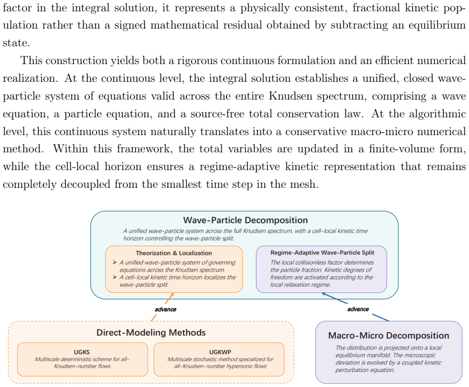
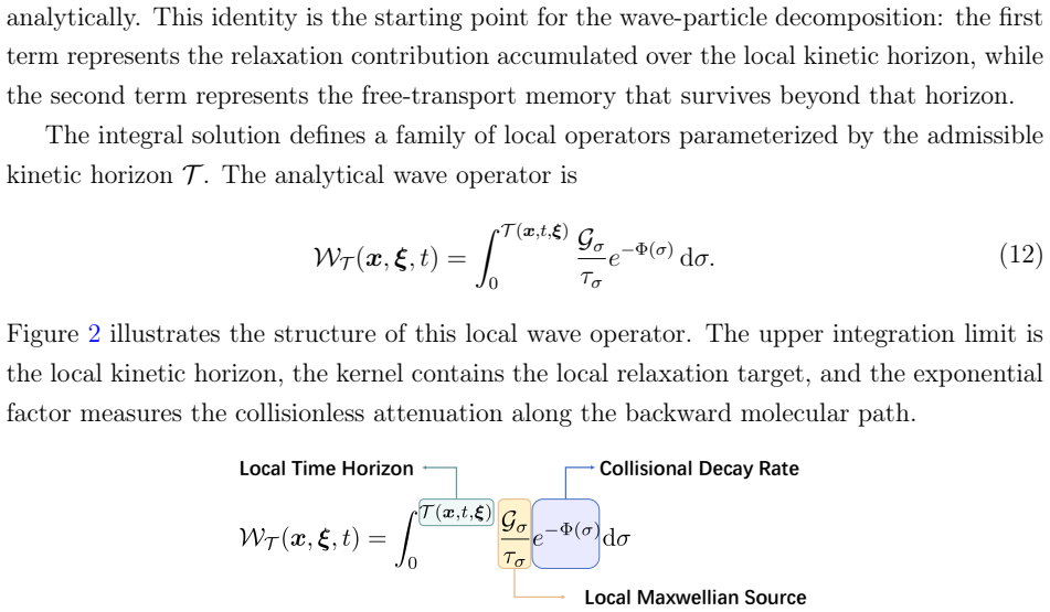
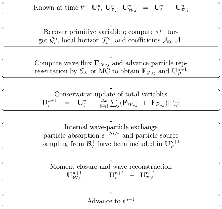
Leveraging the characteristic integral solution of the kinetic relaxation equation, the distribution function is decomposed into a wave component that accumulates analytically within the local horizon and a particle component defined by the collisionless transport that survives beyond the horizon. This yields a closed wave-particle system comprising a source-free total conservation law, a wave equation whose moments produce Euler and Navier-Stokes fluxes with horizon-dependent coefficients, and a particle equation for the remaining non-equilibrium kinetic transport. The formulation holds across the entire Knudsen spectrum and is discretized by advancing total conservative variables with a fi
What carries the argument
The wave-particle decomposition defined around a local evolution timescale and its associated kinetic horizon, which uses the characteristic integral solution to separate the distribution function into an analytically accumulated wave component and a purely kinetic particle component.
Load-bearing premise
The decomposition assumes that a local evolution timescale and associated kinetic horizon can be defined such that the characteristic integral solution accurately separates the analytically accumulated wave component from the surviving kinetic particle component.
What would settle it
A direct numerical comparison in which the wave-particle solution deviates systematically from both the full kinetic reference in the rarefied limit and the Navier-Stokes reference in the continuum limit, for any choice of local horizon, would falsify the unification claim.
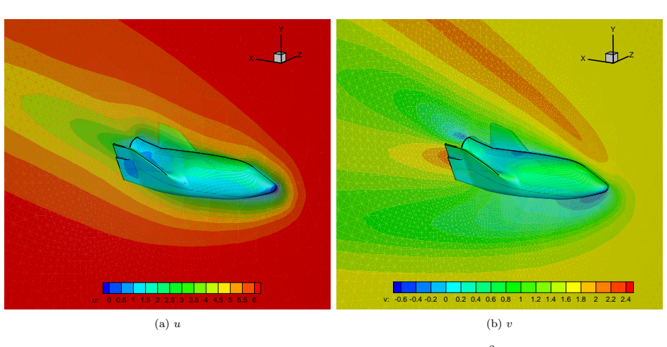
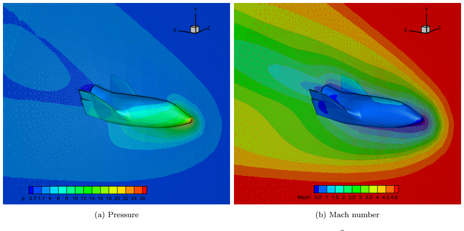
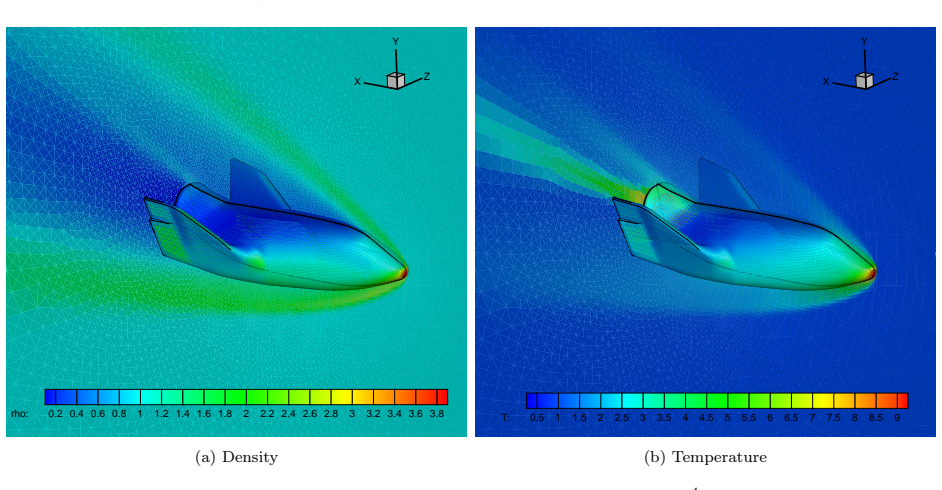
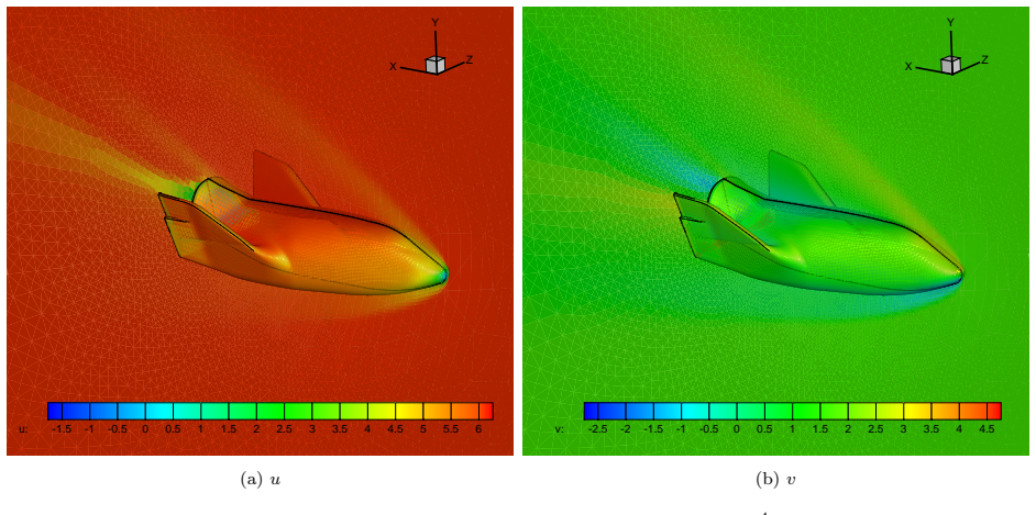
Figures

read the original abstract
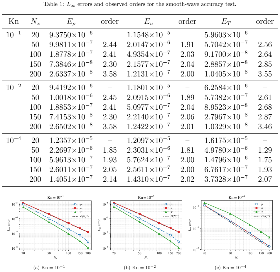
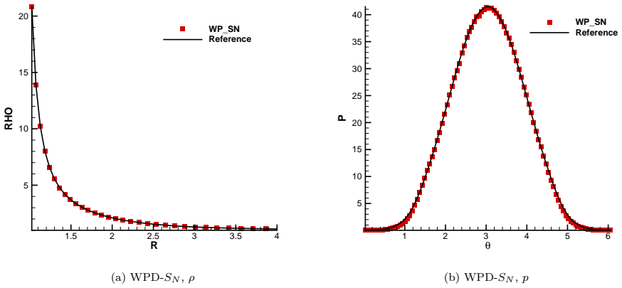
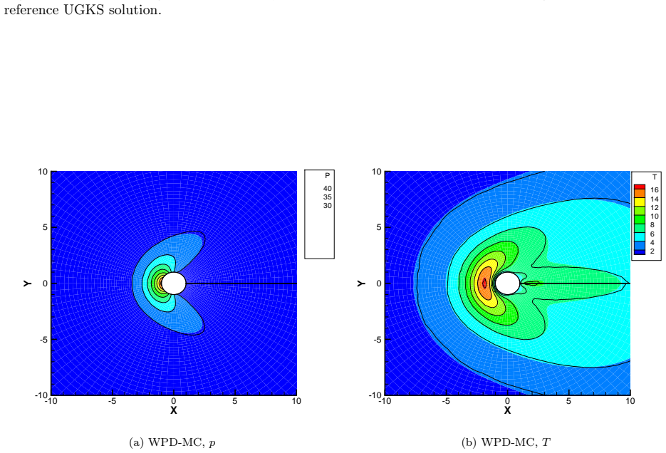
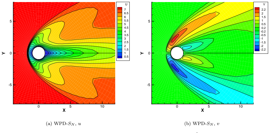
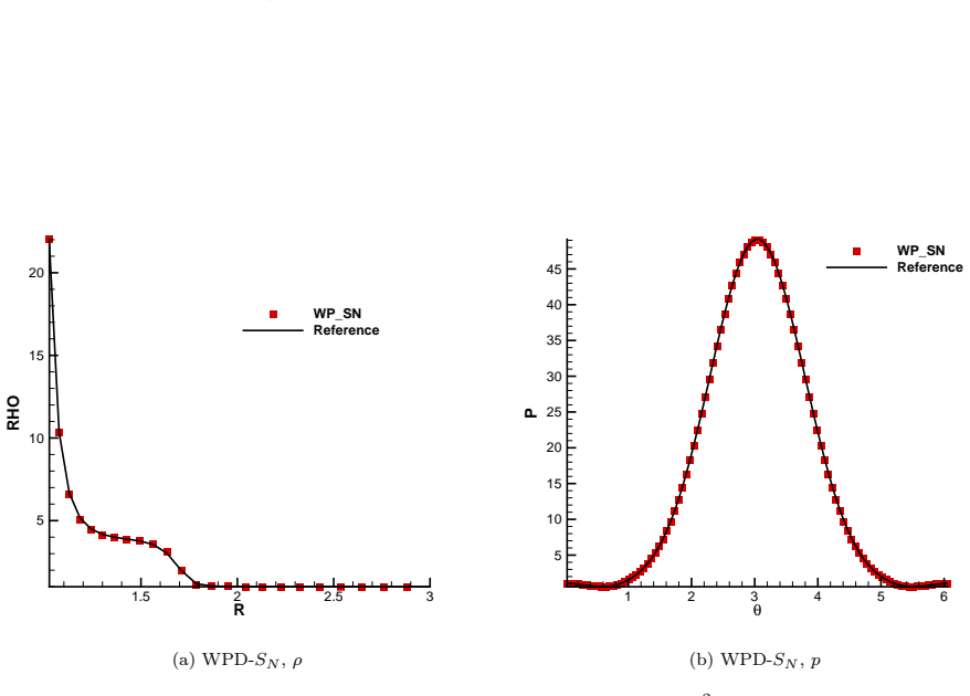
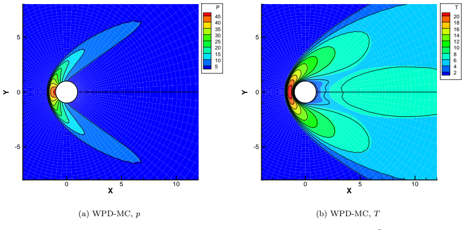
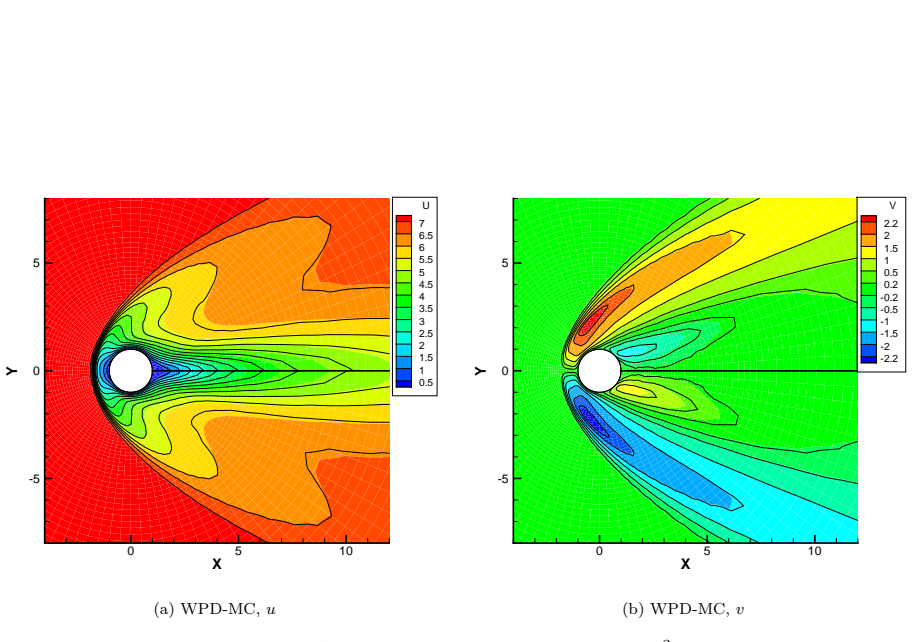
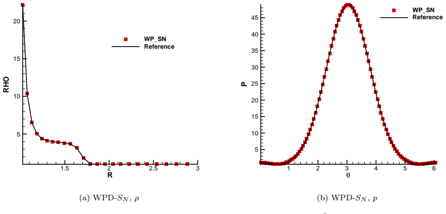
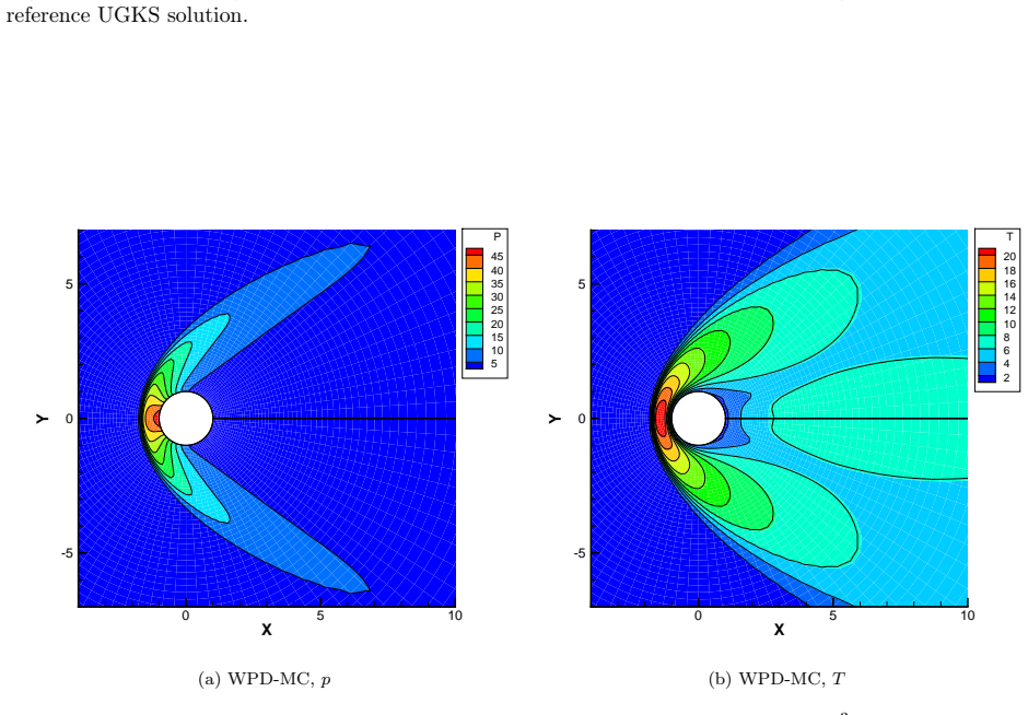
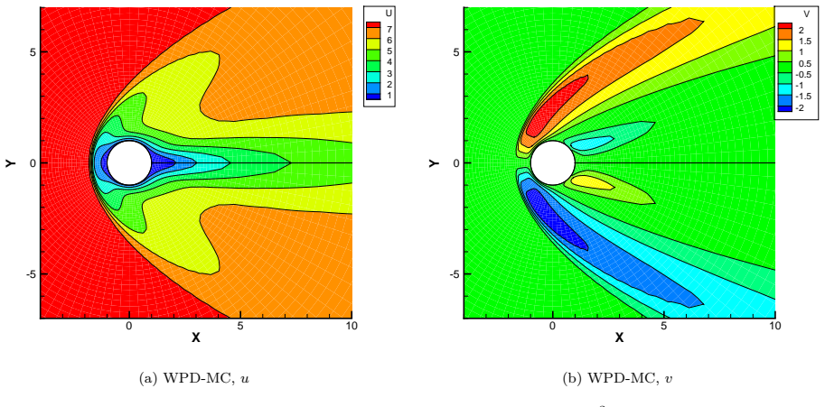
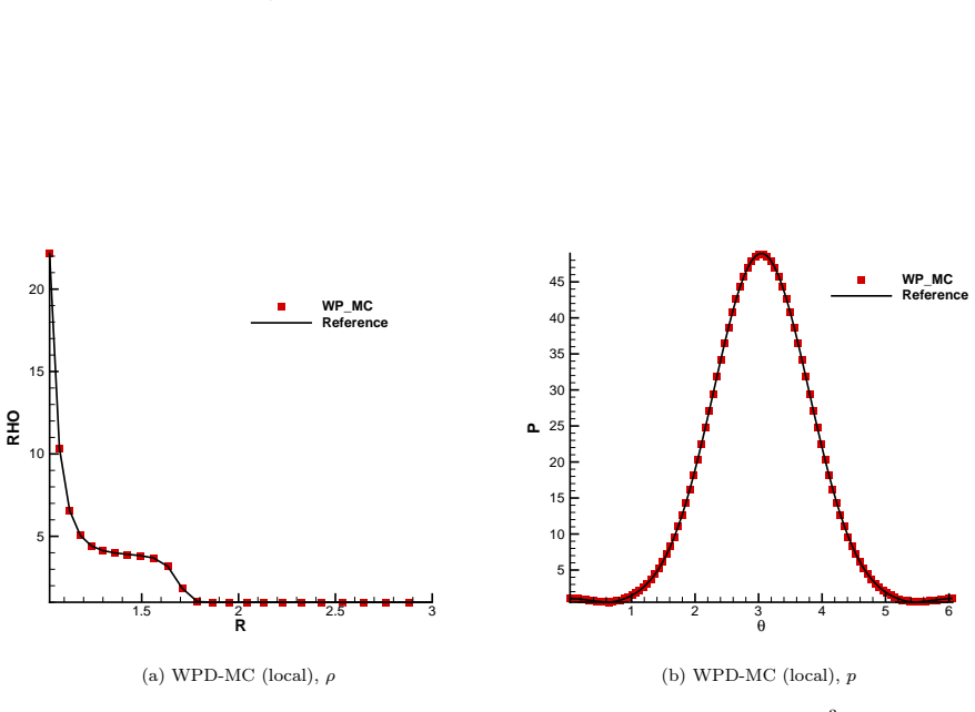
This paper presents a wave-particle decomposition (WPD) for kinetic relaxation equations, formulated around a local evolution timescale and its associated kinetic horizon. By leveraging the characteristic integral solution, we decompose the distribution function into an analytically accumulated wave component and a purely kinetic particle component. The latter is defined by the collisionless transport that survives beyond a prescribed local domain of influence, termed the horizon. This continuous formulation yields a unified wave-particle system valid across the entire Knudsen spectrum, comprising a source-free total conservation law, a wave equation, and a particle equation. The wave operator admits a Chapman--Enskog expansion, whose moments yield Euler and Navier--Stokes fluxes with horizon-dependent coefficients, while the particle equation governs the remaining non-equilibrium kinetic transport. At the algorithmic level, this system is discretized by a conservative macro-micro method. The total conservative variables are advanced by a finite-volume update using the sum of a Navier--Stokes gas-kinetic wave flux and a particle flux computed by either a deterministic discrete-ordinate $(S_N)$ method or a Monte Carlo representation. Unlike the global time-step splitting in the unified gas-kinetic wave-particle (UGKWP) method, the present partition is defined at the PDE level and governed by the local ratio of evolution timescale to relaxation time. The particle component is therefore a fractional kinetic population generated by the collisionless factor of the integral solution. Formal analysis establishes the asymptotic-preserving continuum limit, rarefied-regime consistency, and regime-adaptive scaling of active kinetic degrees of freedom. Numerical tests in one, two, and three dimensions validate the accuracy, multiscale capability, and efficiency of the framework.
Editorial analysis
A structured set of objections, weighed in public.
Referee Report
Summary. The manuscript proposes a wave-particle decomposition (WPD) for kinetic relaxation equations, formulated around a local evolution timescale and associated kinetic horizon. Leveraging the characteristic integral solution, the distribution is partitioned into an analytically accumulated wave component and a collisionless particle component surviving beyond the horizon. This yields a unified continuous system valid across the Knudsen spectrum, consisting of a source-free total conservation law, a wave equation whose moments admit a Chapman-Enskog expansion to horizon-dependent Euler and Navier-Stokes fluxes, and a particle equation for non-equilibrium transport. A conservative macro-micro discretization is introduced, with formal analysis establishing asymptotic-preserving continuum limits, rarefied-regime consistency, and regime-adaptive scaling of kinetic degrees of freedom; numerical tests in 1D-3D are presented.
Significance. If the decomposition is shown to be exact, this PDE-level approach would represent a meaningful extension of prior UGKWP frameworks by eliminating global time-step splitting in favor of a local, horizon-based partition. The claimed formal analysis of the AP property and the conservative macro-micro scheme would be strengths, as would the regime-adaptive particle population that reduces computational cost in near-continuum regions while retaining kinetic fidelity in rarefied zones. Successful validation across dimensions supports potential utility for multiscale problems.
major comments (2)
- [Formulation of the wave-particle system (around the local horizon)] The central claim that the decomposition produces a source-free total conservation law and a unified system valid for arbitrary Knudsen numbers rests on the premise that a local kinetic horizon can be defined such that the characteristic integral exactly separates the wave and particle components without residual sources or regime-dependent errors. An explicit formula for the horizon (in terms of local evolution timescale and relaxation time) and a proof that the separation holds for general initial data must be supplied, as this is load-bearing for the asymptotic-preserving limit and the absence of spurious sources.
- [Chapman--Enskog expansion of the wave operator] § on Chapman-Enskog expansion: the horizon-dependent coefficients in the resulting Euler and Navier-Stokes fluxes are asserted to arise from moments of the wave operator, but the explicit dependence on the horizon parameter and the reduction to standard fluid fluxes in the appropriate limits (e.g., horizon o au or horizon o au/ au) should be derived in detail to confirm consistency with the claimed continuum and rarefied limits.
minor comments (2)
- [Notation and definitions] The notation for the local evolution timescale and the collisionless factor in the integral solution could be clarified with a dedicated definition box or explicit equation reference to aid readers in following the regime-adaptive scaling argument.
- [Discretization and numerical tests] In the numerical section, the description of how the particle flux is computed via S_N or Monte Carlo should include a brief statement on conservation enforcement at the discrete level to match the continuous source-free property.
Simulated Author's Rebuttal
We thank the referee for the careful and constructive review. We address the two major comments below and will revise the manuscript to supply the requested explicit formula, proof, and detailed derivations.
read point-by-point responses
-
Referee: [Formulation of the wave-particle system (around the local horizon)] The central claim that the decomposition produces a source-free total conservation law and a unified system valid for arbitrary Knudsen numbers rests on the premise that a local kinetic horizon can be defined such that the characteristic integral exactly separates the wave and particle components without residual sources or regime-dependent errors. An explicit formula for the horizon (in terms of local evolution timescale and relaxation time) and a proof that the separation holds for general initial data must be supplied, as this is load-bearing for the asymptotic-preserving limit and the absence of spurious sources.
Authors: We agree that an explicit formula and a self-contained proof are necessary to make the claims fully rigorous. The current manuscript defines the horizon via the local ratio of evolution timescale to relaxation time and derives the decomposition from the characteristic integral, but we will add the precise formula (horizon = f(τ_e, τ)) together with a proof that the integral solution separates exactly into wave and particle components for arbitrary initial data, with no residual sources. These additions will be placed in the formulation section to directly support the source-free conservation law and the AP property. revision: yes
-
Referee: [Chapman--Enskog expansion of the wave operator] § on Chapman-Enskog expansion: the horizon-dependent coefficients in the resulting Euler and Navier-Stokes fluxes are asserted to arise from moments of the wave operator, but the explicit dependence on the horizon parameter and the reduction to standard fluid fluxes in the appropriate limits (e.g., horizon o au or horizon o au/au) should be derived in detail to confirm consistency with the claimed continuum and rarefied limits.
Authors: We concur that the explicit dependence and the limiting cases require a more detailed derivation. In the revised manuscript we will expand the Chapman–Enskog section to display the horizon-dependent coefficients explicitly, derive the resulting Euler and Navier–Stokes fluxes from the moments of the wave operator, and prove the recovery of the standard fluid fluxes when the horizon tends to the relaxation time (continuum limit) and when the horizon tends to zero (rarefied limit). revision: yes
Circularity Check
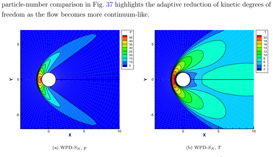
No circularity: PDE-level decomposition is independently formulated
full rationale
The paper defines the wave-particle decomposition directly from the characteristic integral solution of the relaxation equation around a local evolution timescale and kinetic horizon, yielding a source-free conservation law plus separate wave and particle equations. This construction is presented as distinct from the prior UGKWP global time-step splitting, with the new partition governed at the PDE level by the local timescale ratio. Formal analysis of asymptotic-preserving limits and regime-adaptive scaling follows from the stated decomposition and Chapman-Enskog expansion of the wave operator; no step reduces a claimed result to a fitted input, self-citation chain, or definitional renaming. The horizon is an explicit modeling choice in the formulation rather than an output derived from the target properties.
Axiom & Free-Parameter Ledger
axioms (2)
- standard math Characteristic integral solution exists for the kinetic equation
- domain assumption Chapman-Enskog expansion applies to the wave operator
invented entities (1)
-
kinetic horizon
no independent evidence
Reference graph
Works this paper leans on
-
[1]
Boltzmann, Weitere Studien uber das Warmegleichgewicht unter Gasmolekulen, Sitzungsberichte der Kaiserlichen Akademie der Wissenschaften66 (1872) 275–370
L. Boltzmann, Weitere Studien uber das Warmegleichgewicht unter Gasmolekulen, Sitzungsberichte der Kaiserlichen Akademie der Wissenschaften66 (1872) 275–370
-
[2]
Cercignani,The Boltzmann Equation and Its Applications, Springer, New York, 1988
C. Cercignani,The Boltzmann Equation and Its Applications, Springer, New York, 1988
1988
-
[3]
Chapman, T.G
S. Chapman, T.G. Cowling,The Mathematical Theory of Non-Uniform Gases, 3rd ed., Cambridge University Press, Cambridge, 1970
1970
-
[4]
Shakhov, Generalization of the Krook kinetic relaxation equation,Fluid Dyn.3 (1968) 95–96
E.M. Shakhov, Generalization of the Krook kinetic relaxation equation,Fluid Dyn.3 (1968) 95–96
1968
-
[5]
Bird,Molecular Gas Dynamics and the Direct Simulation of Gas Flows, Oxford University Press, Oxford, 1994
G.A. Bird,Molecular Gas Dynamics and the Direct Simulation of Gas Flows, Oxford University Press, Oxford, 1994
1994
-
[6]
Grad, On the kinetic theory of rarefied gases,Commun
H. Grad, On the kinetic theory of rarefied gases,Commun. Pure Appl. Math.2 (1949) 331–407
1949
-
[7]
Pareschi, G
L. Pareschi, G. Russo, Implicit-explicit Runge-Kutta schemes and applications to hy- perbolic systems with relaxation,J. Sci. Comput.25 (2005) 129–155
2005
-
[8]
Filbet, S
F. Filbet, S. Jin, A class of asymptotic-preserving schemes for kinetic equations and related problems with stiff sources,J. Comput. Phys.229 (2010) 7625–7648
2010
-
[9]
Liu, S.-H
T.-P. Liu, S.-H. Yu, Boltzmann equation: Micro-macro decompositions and positivity of shock profiles,Commun. Math. Phys.246 (2004) 133–179
2004
-
[10]
Gamba, S
I.M. Gamba, S. Jin, L. Liu, Micro-macro decomposition based asymptotic-preserving numerical schemes and numerical moments conservation for collisional nonlinear kinetic equations,J. Comput. Phys.382 (2019) 264–290
2019
-
[11]
Xu, J.-C
K. Xu, J.-C. Huang, A unified gas-kinetic scheme for continuum and rarefied flows,J. Comput. Phys.229 (2010) 7747–7764
2010
-
[12]
Xu,Direct Modeling for Computational Fluid Dynamics: Construction and Applica- tion of Unified Gas-Kinetic Schemes, World Scientific, 2014
K. Xu,Direct Modeling for Computational Fluid Dynamics: Construction and Applica- tion of Unified Gas-Kinetic Schemes, World Scientific, 2014
2014
-
[13]
Huang, K
J.-C. Huang, K. Xu, P. Yu, A unified gas-kinetic scheme for continuum and rarefied flows II: multi-dimensional cases,Commun. Comput. Phys.12 (2012) 662–690. 56
2012
-
[14]
C. Liu, K. Xu, A unified gas kinetic scheme for continuum and rarefied flows V: Multi- scale and multi-component plasma transport,Commun. Comput. Phys.22 (2017) 1175– 1223, doi:10.4208/cicp.OA-2017-0102
-
[15]
C. Liu, Z. Wang, K. Xu, A unified gas-kinetic scheme for continuum and rarefied flows VI: Dilute disperse gas-particle multiphase system,J. Comput. Phys.386 (2019) 264– 295, doi:10.1016/j.jcp.2018.12.040
-
[16]
Xu, A gas-kinetic BGK scheme for the Navier-Stokes equations and its connection with artificial dissipation and Godunov method,J
K. Xu, A gas-kinetic BGK scheme for the Navier-Stokes equations and its connection with artificial dissipation and Godunov method,J. Comput. Phys.171 (2001) 289–335
2001
-
[17]
Z. Guo, K. Xu, R. Wang, Discrete unified gas kinetic scheme for all Knudsen number flows: low-speed isothermal case,Phys. Rev. E88 (2013) 033305
2013
-
[18]
C. Liu, Y. Zhu, K. Xu, Unified gas-kinetic wave-particle methods I: Continuum and rarefied gas flow,J. Comput. Phys.401 (2020) 108977
2020
-
[19]
C. Liu, K. Xu, Unified gas-kinetic wave-particle methods IV: multi-species gas mixture and plasma transport,Advances in Aerodynamics(2021) 3:9, https://doi.org/10.1186/s42774-021-00062-1
-
[20]
Fluids31 (2019) 067105
Y.Zhu, C.Liu, C.Zhong, K.Xu, Unifiedgas-kineticwave-particlemethodsII:Multiscale simulation on unstructured mesh,Phys. Fluids31 (2019) 067105
2019
-
[21]
W. Li, C. Liu, Y. Zhu, J. Zhang, K. Xu, Unified gas-kinetic wave-particle methods III: Multiscale photon transport,J. Comput. Phys.408 (2020) 109280
2020
-
[22]
X. Yang, K. Xu, Wave-particle based multiscale modeling and simula- tion of non-equilibrium turbulent flows,Computers & Fluids(2026) 107162, doi:10.1016/j.compfluid.2026.107162
-
[23]
Z. Guo, K. Xu, Y. Zhu, A unified gas-kinetic framework from Boltzmann to Navier- Stokes scales,Advances in Aerodynamics(2026) 8:8, https://doi.org/10.1186/s42774- 025-00252-1
-
[24]
L. Luo, L. Wu, Multiscale simulation of rarefied gas dynamics via di- rect intermittent GSIS-DSMC coupling,Advances in Aerodynamics(2024) 6:22, https://doi.org/10.1186/s42774-024-00188-y
-
[25]
W. Su, L. Zhu, P. Wang, Y. Zhang, L. Wu, Can we find steady-state solutions to multiscale rarefied gas flows within dozens of iterations?J. Comput. Phys.407 (2020) 109245. 57
2020
discussion (0)
Sign in with ORCID, Apple, or X to comment. Anyone can read and Pith papers without signing in.