REVIEW 2 major objections 1 cited by
Time-domain evolution of Lorenz-gauge metric perturbations: taming the $\ell=m=1$ gauge instability
T0 review · 2 major / 0 minor · reviewed 2026-06-26 · grok-4.3
Pith's one-line read An orthogonalized metric perturbation formed from sourced and homogeneous solutions suppresses the linear growth of the m=1 unstable gauge mode.
desk verdict The paper gives a practical numerical fix for the m=1 Lorenz-gauge instability by running a homogeneous solution in parallel and doing occasional orthogonalization, with code supplied for a circular-orbit test case. read the letter →
The pith
A machine-rendered reading of the paper's core claim, the machinery that carries it, and where it could break.
The reading
What carries the argument
The orthogonalized metric perturbation h_ab^ortho, constructed as a linear combination of the sourced MP and a parallel-evolved homogeneous MP, with the combination updated occasionally to enforce orthogonality under a chosen inner product.
What would settle it
A numerical evolution of the orthogonalized MP to very late times that checks whether its amplitude remains bounded or begins growing linearly again.
Extended reading notes
Core claim
For a Schwarzschild-circular-orbit test case, the resulting h_ab^ortho satisfies the O(μ) Einstein equations and Lorenz gauge conditions, remains bounded as t → ∞, and at late (finite) times contains only a small component of the unstable gauge mode. These results hold both with the particle modelled via MP jump conditions and with particle modelled by an effective source.
Load-bearing premise
The m=1 instability can be isolated as a homogeneous gauge mode whose subtraction via the chosen inner product leaves the physical sourced content intact and does not introduce accumulating numerical errors.
Editorial extensions
If this is right
- The orthogonalized perturbation remains bounded as t → ∞.
- It satisfies the O(μ) Einstein equations and Lorenz gauge conditions.
- At late finite times it contains only a small component of the unstable gauge mode.
- The procedure works for both jump-condition and effective-source particle models.
Reading between the lines
- The same orthogonalization step could be tested on non-circular orbits or spinning backgrounds to see whether similar gauge modes appear and can be removed.
- If residual gauge-mode leakage grows with evolution length, the update frequency or inner-product choice might need adjustment to keep errors from accumulating.
- Bounded perturbations of this form could be fed directly into self-force or waveform calculations without additional gauge fixing at late times.
Editorial analysis
A structured set of objections, weighed in public.
Referee Report
Summary. The paper introduces a numerical method to suppress the linearly growing ℓ=m=1 unstable gauge mode that appears in time-domain Lorenz-gauge metric perturbations sourced by a small mass μ orbiting a Schwarzschild black hole. The approach evolves the sourced solution h_ab in parallel with a homogeneous solution h_ab^hom and periodically recomputes coefficients so that an orthogonalized combination h_ab^ortho is orthogonal to h_ab^hom under a chosen inner product. For a circular-orbit test case the resulting h_ab^ortho is reported to satisfy the linearized Einstein equations and Lorenz gauge, to remain bounded at late times, and to contain only a small residual unstable-mode component; the method is demonstrated both with jump conditions and with an effective source, and the code is supplied.
Significance. If the method can be shown to control residual growth over arbitrarily long times without contaminating the physical sourced content, it would remove a practical obstacle to stable, long-duration time-domain calculations of Lorenz-gauge perturbations for EMRIs. The explicit release of the numerical code is a clear strength that supports reproducibility and further testing by the community.
major comments (2)
- [Abstract] Abstract (orthogonalization procedure): the inner product used to enforce orthogonality is never written explicitly, and the update frequency is described only as 'occasional'; without these details it is impossible to assess whether discretization errors in the inner-product evaluation allow a residual unstable mode to grow linearly between updates, which directly affects the central claim that h_ab^ortho remains bounded as t→∞.
- [Abstract] Test-case results (abstract): the demonstration is performed on a single Schwarzschild circular-orbit configuration and reports only that the residual unstable-mode component is 'small' at selected finite times; no error bars, convergence tests with respect to grid spacing or update interval, or quantitative residual norms are provided, leaving the quantitative support for the boundedness claim incomplete.
Simulated Author's Rebuttal
We thank the referee for their careful reading of the manuscript and for the constructive comments. We address each major comment below and indicate the revisions that will be made to strengthen the presentation.
read point-by-point responses
-
Referee: [Abstract] Abstract (orthogonalization procedure): the inner product used to enforce orthogonality is never written explicitly, and the update frequency is described only as 'occasional'; without these details it is impossible to assess whether discretization errors in the inner-product evaluation allow a residual unstable mode to grow linearly between updates, which directly affects the central claim that h_ab^ortho remains bounded as t→∞.
Authors: We agree that the abstract would benefit from greater explicitness on these points. In the revised manuscript we will state the inner product explicitly (the standard L2 inner product over the spatial domain with the usual radial weight factor) and specify the update interval used in the reported runs (every 20M in coordinate time). We will also add a brief sentence noting that this interval is chosen to keep the integrated effect of discretization error on the residual mode below the level that would produce visible linear growth on the timescales shown; the code release allows independent verification of this choice. revision: yes
-
Referee: [Abstract] Test-case results (abstract): the demonstration is performed on a single Schwarzschild circular-orbit configuration and reports only that the residual unstable-mode component is 'small' at selected finite times; no error bars, convergence tests with respect to grid spacing or update interval, or quantitative residual norms are provided, leaving the quantitative support for the boundedness claim incomplete.
Authors: The demonstration is intentionally limited to a single, clean circular-orbit test case to isolate the effect of the orthogonalization procedure. The main text already supplies quantitative residual norms (see the late-time values plotted in Figs. 5–6) and states that the solution remains bounded. To meet the referee’s request we will revise the abstract to include a specific residual-norm figure of merit at late times and a statement that convergence with respect to both grid spacing and update interval has been verified (with the supporting data and code now referenced). Because the evolution is deterministic, conventional error bars are not applicable; the convergence tests themselves serve as the quantitative support. revision: partial
Circularity Check
No circularity: orthogonalization is an explicit numerical procedure demonstrated by direct simulation
full rationale
The paper's central construction is an explicit computational algorithm: evolve the sourced MP and a parallel homogeneous MP, then occasionally form a linear combination that enforces orthogonality under a chosen inner product. This step is introduced as a new method, not derived from prior equations or self-citations, and its properties (satisfying the Einstein equations, remaining bounded, small residual unstable mode) are shown by running the code on a Schwarzschild-circular-orbit test case. No parameter is fitted and then relabeled as a prediction, no uniqueness theorem is imported from the authors' prior work, and the inner-product definition is not reduced to the target result by construction. The derivation chain is therefore self-contained against external benchmarks.
Assumptions & free parameters
assumptions (1)
- domain assumption The m=1 time-domain Lorenz-gauge instability is a homogeneous gauge mode that can be isolated and removed by orthogonalization without corrupting the sourced physical solution.
Cite this review
Pith. "Pith review of Time-domain evolution of Lorenz-gauge metric perturbations: taming the $\ell=m=1$ gauge instability." pith.science (2026). https://pith.science/paper/5ZWQ3C4K
@misc{pith2026260627016,
  author       = {Pith},
  title        = {Pith review of: Time-domain evolution of Lorenz-gauge metric perturbations: taming the $\ell=m=1$ gauge instability},
  year         = {2026},
  howpublished = {\url{https://pith.science/paper/5ZWQ3C4K}},
  note         = {Machine review of arXiv:2606.27016}
}
abstract
Calculating the spacetime metric perturbation (MP) sourced by a small "particle" of mass $\mu M$ (with $0 < \mu \ll 1$) moving in a Schwarzschild or Kerr "background" black hole spacetime of mass $M$ is a longstanding research area in general relativity. This calculation also has an important astrophysical motivation as a major step in calculating the gravitational waves emitted by an extreme-mass-ratio inspiral system. Here I consider the specific problem of the time-domain calculation of the $\mathcal{O}(\mu)$ Lorenz-gauge MP $h_{ab}$ sourced by the particle. Decomposing the Schwarzschild-background MP into $e^{im\phi}$ modes, Dolan and Barack [Phys. Rev. D 87, 084066 (2013), arXiv:1211.4586] found that the $m=1$ time-domain Lorenz-gauge MP generically contains an \emph{unstable gauge mode} which grows linearly with time. Here I demonstrate a method for computing a Lorenz-gauge time-domain evolution which is mostly free of this gauge mode. This method computes an "orthogonalized" MP $h_{ab}^\text{ortho}$ as a linear combination of the sourced MP and a homogeneous MP $h_{ab}^\text{hom}$ (evolved in parallel with the sourced MP). The linear combination is updated "occasionally" to make $h_{ab}^\text{ortho}$ orthogonal to $h_{ab}^\text{hom}$ with respect to a chosen inner product on MPs. I show that, for a Schwarzschild-circular-orbit test case, the resulting $h_{ab}^\text{ortho}$ satisfies the $\mathcal{O}(\mu)$ Einstein equations and Lorenz gauge conditions, remains bounded as $t \to \infty$, and at late (finite) times contains only a small component of the unstable gauge mode. These results hold both with the particle modelled via MP jump conditions and with particle modelled by a "effective source". My numerical code for obtaining all of these results is included with this paper, and will be deposited in the Black Hole Perturbation Toolkit.
Figures


Figures from the paper (21 more)






Forward citations
Cited by 1 Pith paper
-
Schwarzschild perturbations in Lorenz gauge via elliptic differential equations
First frequency-domain m-mode calculation of Schwarzschild metric perturbations in Lorenz gauge, solving ten coupled elliptic PDEs and matching known energy fluxes to about four digits.
Reference graph
Works this paper leans on
-
[1]
occasionally
In particular, the orthogonalized ¯h(I) remain bounded throughout the evolution, and their Lorenz gauge constraints Y (1, 2, 3) and rescaled Einstein tensor ˜Gab are smsll at late times. The particle-orbit-period oscillations are clearly visible in the movie; the evolution is not dominated by the unstable mode. Figure 11 shows the time evolution of the un...
2014
-
[2]
Integrating ( A1) from xp − ǫ to xp + ǫ and taking the limit ǫ → 0 gives the jump in ∂xu as [u′]p = lim ǫ→ 0 { u′(xp + ǫ) − u′(xp − ǫ) } = s(t)
General Formalism Slightly generalizing the BL05 evolution equations, consider a 1+1-dimensional linear wave equation with a δ-function source, − ∂ttu + ∂xxu + T(x)∂tu + X(x)∂xu + V(x)u = s(t) , (A1) where for the remainder of this appendix only, x := r∗ , N > 0 is an integer, s(t) is an N -element column vector, T(x), X(x), and V(x) are N × N coefficient m...
-
[3]
don’t repeat yourself
Application to the ¯h(Iℓm) evolution equations To apply the above formalism to the BL05 evolution equations ( 3.7), take N to be the number of nontriv- ial ¯h(Iℓm) (N = 6 for the ℓ= m = 1 case which is my focus here), u to be an N -element column vector of those non- trivial ¯h(Iℓm), and take s(t) to be an N -element column vector of the nontrivial compon...
-
[4]
I compute these by numerically inverting the tortise-coordinate defini- tion ( 3.2)
Computing r(r∗ ) Since I use a numerical grid uniform in r∗ , computing various coefficients at the grid points requires knowing the r coordinates of the grid points. I compute these by numerically inverting the tortise-coordinate defini- tion ( 3.2). To do this, I define y = ln ( r 2M − 1 ) (B1) x∗ = r∗ 2M , (B2) so that r∗ = r + 2M y and r = 2 M (1 + ey). (...
-
[5]
crosses the particle
Notation for the remainder of this Appendix Throughout the remainder of this appendix, I suppress the indices (Iℓm) ab , and I use a lower-case Latin typewriter- font i to index grid functions. When describing finite-difference molecules (stencils), I use a lower-case Latin typewriter-font m to index the molecule coefficients, so that a generic finite-differenc...
-
[6]
(B9) I use 4th order centered finite differencing on a uniform-in-r∗ grid to approximate the spatial derivatives in the RHS(vacuum) definition ( 3.7c) and the M operator
Main finite differencing For each (ℓ, m ), I use a 4th-order Runge-Kutta method of lines scheme to time-integrate of the ¯h(I) evolution equations ( 3.7), written in the 1st-order-in-time form ∂t (¯h(I), ∂ t¯h(I)) = ( ∂t¯h(I), RHS(total)(¯h(I), ∂ t¯h(I)) ) . (B9) I use 4th order centered finite differencing on a uniform-in-r∗ grid to approximate the spatial d...
-
[7]
(B10) All the results presented here use the dissipation coeffi- cient ǫ = 0
Dissipation To reduce numerical noise, I add an additional dissi- pation term ǫD(¯h) to the right hand side of ( 3.7c) at 25 selected grid points, where the dissipation operator D is the 6th-order Kreiss-Oliger dissipation operator (Rinne [28, appendix C]) with finite-difference molecule D = 1 64 ∆ r∗ [ +1 − 6 +15 − 20 +15 − 6 +1 ] . (B10) All the results p...
-
[8]
adjusted
Source Terms Despite the major conceptual differences between the point-particle and effective-source particle models, their implementations at the level of finite differencing are actually mostly similar. In both cases, for each finite-differencing operation at a grid point i, the code first tests • for a point-particle model, whether or not the finite difference...
Show all 60 references
-
[9]
116M instead of P/ 4 ≈ 30
Shorter Orthogonalization Time Spacing To show the effect of changing the orthogonalization time spacing ∆ t(ortho), here I briefly present the esrc- ortho-P12 evolution, which is identical to the esrc-ortho- P4 evolution presented in section IV C except that the orthogonalizati...
-
[10]
Changing the definition of λ( occasionally updated ) to be less oscillatory would be useful: 0 0.2 0.4 0.6 0.8 1 0 200 400 600 800 1000 |〈– h(ortho), – h(hom)〉| t (M) FIG
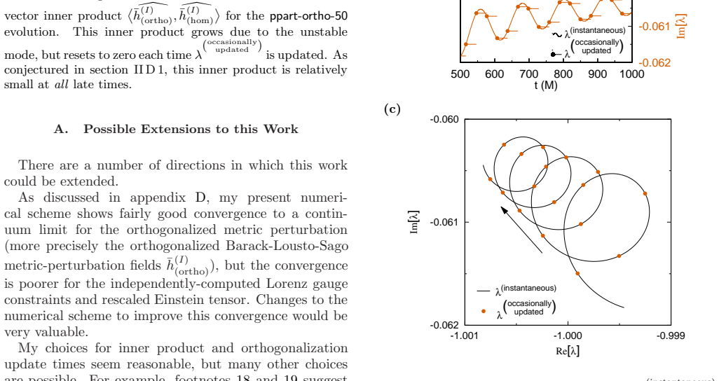
Orbit Averaging Figures 4 and 8 show that after an initial transient, λ (instantaneous) – and thus λ(occasionally updated ) – tends to oscillate in a slowly-decaying spiral pattern in the complex plane, with oscillation period equal to the particle’s orbital period P . Changin...
-
[11]
The scale is the same as that of figure 9 (which shows the esrc-ortho-P4 evolution)
116M . The scale is the same as that of figure 9 (which shows the esrc-ortho-P4 evolution). In comparison to that evolution, here the unit-vector inner product is much small er (≲ 0. 1) at late times. 0 5 10 15 0 200 400 600 800 1000 10-8 10-6 10-4 10-2 100 ||– h(I)|| ||Y(1,2,3...
-
[12]
gradual-turnon function
Gradual Turnon of the Puncture and Effective Source As noted in section III B 2, if the initial data doesn’t already satisfy the jump conditions ( 3.9) across the worldtube boundary, the dynamical evolution generates high-spatial-frequency noise in the process of driving the fie...
-
[13]
In order for the unstable gauge mode to still be mostly cancelled, λ (fixed) should be fairly close to λ (instantaneous)
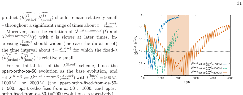
Using a Fixed λ Another way to reduce the jumps in λ( occasionally updated ) is to never update λ(occasionally updated ), i.e., to choose λ(occasionally updated ) to actually be some fixed (time-independent) constant λ (fixed) . In order for the unstable gauge mode to still be m...
-
[14]
Compute a “base” orthogonalized evolution (pos- sibly using orbit-averaging) for some time period t ∈ [0, t (base) max ]
-
[15]
Choose λ (fixed) to be λ (instantaneous)(t(base) max ), λ (orbit averaged) (t(base) max ), or some series acceleration (e.g., the Aitken, Richardson, or Shanks transformation) of the time sequence of λ (instantaneous) or λ (orbit averaged) in the base orthogonalized evolution
-
[16]
relatively small
Now compute a new “fixed- λ” approximately- orthogonalized evolution (starting from t = 0) using λ(occasionally updated )(t) = λ (fixed) . The goal is that the fixed- λ metric perturbation should contain only a relatively small component of the unstable mode throughout some “usef...
2000
-
[17]
Parts (a) and (c) show ¯h(I) (lo) − ¯h(I) (hi) as a function of time for each evolution and each resolution pair
Convergence of ¯h(I) (ortho) Figure 22 shows the convergence of ¯h(I) (lo) − ¯h(I) (hi) for the ppart-ortho-50 and esrc-ortho-P4 evolutions. Parts (a) and (c) show ¯h(I) (lo) − ¯h(I) (hi) as a function of time for each evolution and each resolution pair. Parts (b...
2000
-
[18]
In each fig- ure, parts (a) and (c) show · as a function of time for each evolution and each resolution
Convergence of the Lorenz gauge constraints Figure 23 shows the convergence of Y (1, 2, 3) for the ppart-ortho-50 and esrc-ortho-P4 evolutions. In each fig- ure, parts (a) and (c) show · as a function of time for each evolution and each resolution. Parts (b) and (...
-
[19]
In each figure, parts (a) and (c) show · as a function of time for each evolution and each resolution
Convergence of the rescaled Einstein tensor Figure 24 shows the convergence of ˜Gab for the ppart- ortho-50 and esrc-ortho-P4 evolutions. In each figure, parts (a) and (c) show · as a function of time for each evolution and each resolution. Parts (b) and (d) sho...
-
[20]
Convergence Summary Figure 22 shows that in both the ppart-ortho-50 and esrc-ortho-P4 evolutions, ¯h(I) (lo) − ¯h(I) (hi) converges smoothly (to zero) with increasing resolution ( decreasing (∆ r∗ )(lo) ) . However, figures 23 and 24 show significant limitations and non-u...
-
[21]
( bhptoolkit.org), 2026
Black Hole Perturbation Toolkit. ( bhptoolkit.org), 2026
2026
-
[22]
Introduction to 3 + 1 Numerial Rela- tivity
Miguel Alcubierre. Introduction to 3 + 1 Numerial Rela- tivity. Oxford U.P., Oxford, U.K., 1986
1986
-
[23]
Self-force effects on the marginally bound zoom-whirl orbit in Schwarzschild spacetime
Leor Barack, Marta Colleoni, Thibault Damour, Soichiro Isoyama, and Norichika Sago. Self-force effects on the marginally bound zoom-whirl orbit in Schwarzschild spacetime. Phys. Rev. D , 100:124015, Dec 2019
2019
-
[24]
Golbourn
Leor Barack and Darren A. Golbourn. Scalar-field per- turbations from a particle orbiting a black hole using numerical evolution in 2+1 dimensions. Phys. Rev. D , 76(4):044020, Aug 2007
2007
-
[25]
Leor Barack and Carlos O. Lousto. Perturbations of 35 (a) ppart-ortho-50 evolution 10-10 10-8 10-6 10-4 10-2 100 0 500 1000 1500 2000 ||Y(1,2,3)|| t (M) ∆r*=M/2 ∆r*=M/3 ∆r*=M/4 ∆r*=M/6 ∆r*=M/8 ∆r*=M/12 ∆r*=M/16 ∆r*=M/24 ∆r*=M/32 (b) ppart-ortho-50 evolution 10-10 10-9 10-8 10-...
2000
-
[26]
Gravitational self-force on a particle in circular orbit around a Schwarzschild black hole
Leor Barack and Norichika Sago. Gravitational self-force on a particle in circular orbit around a Schwarzschild black hole. Phys. Rev. D , 75(6):064021, 2007
2007
-
[27]
Gravitational self- force correction to the innermost stable circular orbit of a Schwarzschild black hole
Leor Barack and Norichika Sago. Gravitational self- force correction to the innermost stable circular orbit of a Schwarzschild black hole. Phys. Rev. Lett. , 102(19): 191101, 2009
2009
-
[28]
Gravitational self-force on a particle in eccentric orbit around a Schwarzschild black hole
Leor Barack and Norichika Sago. Gravitational self-force on a particle in eccentric orbit around a Schwarzschild black hole. Phys. Rev. D , 81(8):084021, Apr 2010
2010
-
[29]
Beyond the geodesic approximation: conservative effects of the gravitational self-force in eccentric orbits around a Schwarzschild blac k hole
Leor Barack and Norichika Sago. Beyond the geodesic approximation: conservative effects of the gravitational self-force in eccentric orbits around a Schwarzschild blac k hole. Phys. Rev. D , 83(8):084023, Apr 2011
2011
-
[30]
Post-Newtonian theory for gravitational waves
Luc Blanchet. Post-Newtonian theory for gravitational waves. Living Reviews in Relativity , 27(4), 2024
2024
-
[31]
Elements of Numerical Relativity: From Einstein ’s Equations to Black Hole Simulations
Carles Bona and Carlos Palenzuela-Luque. Elements of Numerical Relativity: From Einstein ’s Equations to Black Hole Simulations . Number 673 in Lecture Notes in Physics. Springer-Verlag, 1st edition, 2005
2005
-
[32]
Choptuik
Matthew W. Choptuik. Consistency of finite-difference solutions to Einstein’s equations. Phys. Rev. D , 44(10): 3124–3135, 1991
1991
-
[33]
Low multipole con- tributions to the gravitational self-force
Steven Detweiler and Eric Poisson. Low multipole con- tributions to the gravitational self-force. Phys. Rev. D , 69:084019, Apr 2004
2004
-
[34]
Steven Detweiler and Bernard F. Whiting. Self-force via a Green’s function decomposition. Phys. Rev. D , 67(2): 024025, Jan 2003
2003
-
[35]
Dolan and Leor Barack
Sam R. Dolan and Leor Barack. Self force via m-mode regularization and 2+1 D evolution: III. Gravitational field on Schwarzschild spacetime. Phys. Rev. D , 87: 084066, Apr 2013
2013
-
[36]
Dolan, Leanne Durkan, Chris Kavanagh, and Barry Wardell
Sam R. Dolan, Leanne Durkan, Chris Kavanagh, and Barry Wardell. Metric perturbations of Kerr spacetime in Lorenz gauge: circular equatorial orbits. Class. Quant. Grav., 41(15):155011, 2024. 36 (a) ppart-ortho-50 evolution 10-8 10-6 10-4 10-2 100 102 0 500 1000 1500 2000 ||~ Ga...
2024
-
[37]
The Sage project: Unifying free mathematical software to create a viable alternative to Magma, Maple, Mathematica and Matlab
Bur¸ cin Er¨ ocal and William Stein. The Sage project: Unifying free mathematical software to create a viable alternative to Magma, Maple, Mathematica and Matlab. In Komei Fukuda, Joris van der Hoeven, Michael Joswig, and Nobuki Takayama, editors, ICMS 2010: Proceedings of the...
2010
-
[38]
The post- Newtonian approximation for relativistic compact bina- ries
Toshifumi Futamase and Yousuke Itoh. The post- Newtonian approximation for relativistic compact bina- ries. Living Reviews in Relativity , 10(1):2, 2007
2007
-
[39]
What every computer scientist should know about floating-point arithmetic
David Goldberg. What every computer scientist should know about floating-point arithmetic. ACM Computing Surveys, 23(1):5–48, 1991
1991
-
[40]
Golub and Charles F
Gene H. Golub and Charles F. Van Loan. Matrix Com- putations. Johns Hopkins University Press, Baltimore, MD, USA, 4th edition, 2013
2013
-
[41]
Tensor calculus with open-source software: the SageMan- ifolds project
´Eric Gourgoulhon, Michal Bejger, and Marco Mancini. Tensor calculus with open-source software: the SageMan- ifolds project. Journal of Physics: Conference Series , 600:012002, Apr 2015
2015
-
[42]
Symbolic ten- sor calculus on manifolds: a SageMath implementation , pages 1–54
´Eric Gourgoulhon and Marco Mancini. Symbolic ten- sor calculus on manifolds: a SageMath implementation , pages 1–54. Number 1 in Les cours du CIRM. CIRM, 2018
2018
-
[43]
Green, Stefan Hollands, Laura Sberna, Vahid Toomani, and Peter Zimmerman
Stephen R. Green, Stefan Hollands, Laura Sberna, Vahid Toomani, and Peter Zimmerman. Conserved currents for a Kerr black hole and orthogonality of quasinormal modes. Physical Review D , 107(6):064030, Mar 2023
2023
-
[44]
The Pragmatic Pro- grammer: From Journeyman to Master
Andrew Hunt and David Thomas. The Pragmatic Pro- grammer: From Journeyman to Master . Addison-Wesley, Reading, MA, USA, 2nd edition, 2019
2019
-
[45]
Katz, Alvin J
Michael L. Katz, Alvin J. K. Chua, Lorenzo Speri, 37 Niels Warburton, and Scott A. Hughes. Fast extreme- mass-ratio-inspiral waveforms: New tools for millihertz gravitational-wave data analysis. Physical Review D , 104 (6), Sep 2021
2021
-
[46]
Waveform modelling for the Laser Interferometer Space Antenna
LISA Consortium Waveform Working Group. Waveform modelling for the Laser Interferometer Space Antenna
-
[47]
An axisymmetric evolution code for the Einstein equations on hyperboloidal slices
Oliver Rinne. An axisymmetric evolution code for the Einstein equations on hyperboloidal slices. Class. Quant. Grav., 27(3), 15 January 2010
2010
-
[48]
Hamiltonian formulation of general relativity and post-Newtonian dy- namics of compact binaries
Gerhard Sch¨ afer and Piotr Jaranowski. Hamiltonian formulation of general relativity and post-Newtonian dy- namics of compact binaries. Living Reviews in Relativity , 27(2), 2024
2024
-
[49]
SAGE: System for Algebra and Geometry Experimentation
William Stein and David Joyner. SAGE: System for Algebra and Geometry Experimentation. ACM SIGSAM Bulletin, 39(2):61–64, 2005
2005
-
[50]
Teukolsky
Saul A. Teukolsky. The Kerr metric. Class. Quant. Grav., 32(124006), 2014
2014
-
[51]
SageMath, the Sage Math- ematics Software System (Version 10.5.beta0) , 2024
The Sage Developers. SageMath, the Sage Math- ematics Software System (Version 10.5.beta0) , 2024. https://www.sagemath.org
2024
-
[52]
A 3+1 computational scheme for dynamic spherically symmetric black hole spacetimes – I: Initial data
Jonathan Thornburg. A 3+1 computational scheme for dynamic spherically symmetric black hole spacetimes – I: Initial data. Phys. Rev. D , 59(10):104007, 1999
1999
-
[53]
Scalar self-force for highly eccentric equatorial orbits in Kerr spacetime
Jonathan Thornburg and Barry Wardell. Scalar self-force for highly eccentric equatorial orbits in Kerr spacetime. Phys. Rev. D , 95:084043, Apr 2017
2017
-
[54]
Regularization of fields for self-force problems in curved spacetime: Foundations and a time-domain application
Ian Vega and Steven Detweiler. Regularization of fields for self-force problems in curved spacetime: Foundations and a time-domain application. Phys. Rev. D , 77(8): 084008, Apr 2008
2008
-
[55]
Robert M. Wald. General relativity . The University of Chicago Press, Chicago, 1984
1984
-
[56]
Self-force: Computational strategies
Barry Wardell. Self-force: Computational strategies. In Dirk Puetzfeld, Claus L¨ ammerzahl, and Bernard Schutz, editors, Equations of Motion in Relativistic Gravity , vol- ume 179 of Fundamental Theories of Physics , pages 487–
-
[57]
Springer International Publishing, 2015
2015
-
[58]
LorenzGauge1DEffectiveSource: Numeri- cal code to compute a Lorenz-gauge 1-dimensional effec- tive source, 2015
Barry Wardell. LorenzGauge1DEffectiveSource: Numeri- cal code to compute a Lorenz-gauge 1-dimensional effec- tive source, 2015
2015
-
[59]
Barry Wardell, Chris Kavanagh, and Sam R. Dolan. Sourced metric perturbations of Kerr spacetime in Lorenz gauge. Class. Quant. Grav. , 42(20):205007, 2025
2025
-
[60]
Metric recon- struction from Weyl scalars
Bernard F Whiting and Larry R Price. Metric recon- struction from Weyl scalars. Class. Quant. Grav. , 22 (15):S589–S604, 2005
2005
Reviewed June 26, 2026 · model on record in the stance chip above.
Discussion (0). Continue with ORCID to comment.