PAC-Bayesian Certificates for Quadratic Closed-Loop Control

Domagoj Herceg

arxiv: 2606.28281 · v1 · pith:7O33LLMOnew · submitted 2026-06-26 · 📡 eess.SY · cs.LG· cs.SY

PAC-Bayesian Certificates for Quadratic Closed-Loop Control

Domagoj Herceg This is my paper

Pith reviewed 2026-06-29 02:45 UTC · model grok-4.3

classification 📡 eess.SY cs.LGcs.SY

keywords PAC-BayesSystem Level Synthesisquadratic controlclosed-loop certificationfinite-sample guaranteeslearning-based controlGaussian disturbancessensitivity bounds

0 comments

The pith

System Level Synthesis makes quadratic trajectory costs amenable to explicit PAC-Bayes-Chernoff certification for closed-loop responses.

A machine-rendered reading of the paper's core claim, the machinery that carries it, and where it could break.

The paper develops finite-sample guarantees for learning-based control by applying PAC-Bayesian methods to quadratic trajectory costs, which are typically unbounded and non-Lipschitz. It employs System Level Synthesis parameterization to expose the closed-loop trajectory map of linear systems directly, yielding a family of PAC-Bayes-Chernoff certificates for posterior distributions over feasible closed-loop responses. For Gaussian disturbance trajectories with arbitrary covariance, an exact one-sided Gaussian transform and a tractable quadratic upper bound are derived through closed-loop sensitivity quantities. The convex quadratic form of the SLS loss transfers the certificate to the posterior mean response, supporting deterministic deployment while retaining the stochastic posterior in the bound. A data-driven version of the bound produces a learning algorithm that improves held-out cost and reduces closed-loop sensitivity in low-data regimes.

Core claim

System Level Synthesis parameterization exposes the closed-loop trajectory map directly and renders the quadratic control loss amenable to explicit certification, producing PAC-Bayes-Chernoff certificates for posteriors over feasible responses; for Gaussian disturbances the loss admits an exact one-sided transform and quadratic upper bound via sensitivity quantities, the convex form transfers the certificate to the posterior mean, and a data-driven bound supports mean-response deployment from finite samples.

What carries the argument

System Level Synthesis parameterization of closed-loop trajectory maps, which renders the quadratic loss certifiable through closed-loop sensitivity quantities.

If this is right

PAC-Bayes-Chernoff certificates apply directly to posterior distributions over feasible closed-loop responses.
The certificate on the stochastic posterior transfers to the deterministic mean response for control deployment.
A data-driven bound replaces the oracle bound and yields a learning algorithm for control selection.
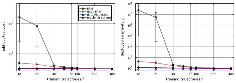
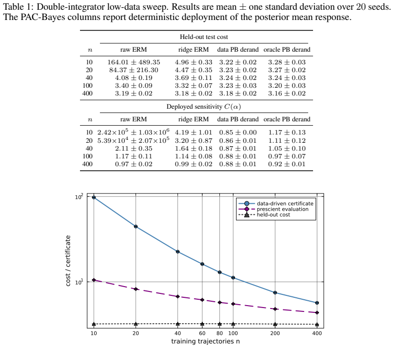
Minimizing the bound produces sensitivity-aware finite-sample regularization that improves held-out cost.

Where Pith is reading between the lines

These are editorial extensions of the paper, not claims the author makes directly.

The sensitivity quantities in the bound could guide controller design choices that trade performance for robustness in other linear systems.
The data-driven bound construction may allow incremental updates when new trajectory samples arrive online.
If similar parameterizations exist for other cost structures, the same transfer from posterior to mean could apply beyond quadratics.

Load-bearing premise

The quadratic control loss admits an exact one-sided Gaussian transform and a tractable quadratic upper bound expressed through closed-loop sensitivity quantities for Gaussian disturbance trajectories with arbitrary covariance.

What would settle it

If the PAC-Bayes bound computed from the posterior fails to upper-bound the true quadratic cost of the posterior mean response on held-out Gaussian disturbance trajectories in the double-integrator experiments.

Figures

Figures reproduced from arXiv: 2606.28281 by Domagoj Herceg.

**Figure 1.** Figure 1: Double-integrator low-data sweep with p = 110. Left: held-out test cost. Right: deterministic deployed sensitivity. Raw ERM is highly unstable when n ≪ p. Ridge regularization stabilizes point optimization, but the data-driven derandomized PAC-Bayes mean response achieves substantially lower test cost and lower sensitivity in the low-data regime. As n increases, all methods converge, indicating that the a… view at source ↗

**Figure 2.** Figure 2: Numerical certificate tightness for the learned data-driven posterior. Curves show means [PITH_FULL_IMAGE:figures/full_fig_p012_2.png] view at source ↗

read the original abstract

PAC-Bayesian bounds provide finite-sample guarantees for data-dependent randomized predictors, but applying them to learning-based control is difficult because the natural objective is a quadratic trajectory cost. Such losses are unbounded, non-Lipschitz , and lead to response-dependent Chernoff terms. We employ System Level Synthesis parameterization, which exposes the closed-loop trajectory map of a linear system directly and makes the quadratic control loss amenable to explicit certification. Moreover, we provide a set of PAC-Bayes-Chernoff certificates for posterior distributions over feasible closed-loop responses. For Gaussian disturbance trajectories with arbitrary covariance, we derive an exact one-sided Gaussian transform and a tractable quadratic upper bound expressed through closed-loop sensitivity quantities. We also derive a posterior-localized surrogate for settings where pointwise closed-loop response certificates are unavailable or have support related admissibility issues. Although PAC-Bayes certifies a non-degenerate posterior, the convex quadratic form of the SLS loss transfers the certificate to the posterior mean response. We present a deterministic mean response deployment result that is particularly suitable for control while retaining the stochastic posterior in the bound. Additionally, we provide a data-driven bound for this deployment, transitioning away from an oracle bound. Minimizing this bound naturally results in a learning algorithm for control selection from data. Numerical experiments on a double integrator show that the algorithm acts as a sensitivity-aware finite-sample regularizer, improving held-out cost and reducing closed-loop sensitivity in the low-data regime

Editorial analysis

A structured set of objections, weighed in public.

Desk editor's note, referee report, simulated authors' rebuttal, and a circularity audit. Tearing a paper down is the easy half of reading it; the pith above is the substance, this is the friction.

Desk Editor's Note private letter to a colleague

SLS parameterization plus PAC-Bayes-Chernoff yields certificates for quadratic closed-loop costs, but the exact one-sided Gaussian transform for arbitrary covariance needs direct checking.

read the letter

The paper's core contribution is a set of PAC-Bayes certificates for posteriors over SLS-parameterized closed-loop responses, with the quadratic trajectory cost handled via an exact one-sided Gaussian transform and a tractable quadratic upper bound in closed-loop sensitivities. It also gives a deterministic mean-response deployment result that keeps the stochastic posterior in the bound, plus a data-driven version that produces a learning algorithm. The double-integrator experiments indicate the bound functions as a sensitivity-aware regularizer in the low-data regime.

This is new relative to prior PAC-Bayes control work, which used different parameterizations or bounded losses. The approach is formally grounded in standard SLS and PAC-Bayes-Chernoff machinery, with low circularity burden, and the abstract framing shows honest engagement with the unbounded-loss problem.

The main soft spot is the stress-test concern: whether the Gaussian transform remains exact and uniformly tractable for general posteriors and arbitrary disturbance covariance without hidden restrictions on the effective matrix, the Chernoff parameter, or posterior support. The abstract claims an exact transform and a posterior-localized surrogate for admissibility issues, but the full derivations must confirm this holds without post-hoc choices or domain restrictions. If it does, the claims are solid; if not, generality is narrower than stated.

The work is for researchers in safe learning-based control who need finite-sample guarantees rather than simulation checks. A reader focused on certified linear controller selection from data would find the explicit forms and deployment result useful.

It deserves peer review to verify the transform step and the experiments.

Referee Report

2 major / 2 minor

Summary. The paper claims that System Level Synthesis (SLS) parameterization renders quadratic trajectory costs amenable to explicit PAC-Bayes-Chernoff certification for linear systems. It derives a set of certificates for posteriors over feasible closed-loop responses, including an exact one-sided Gaussian transform and tractable quadratic upper bound (expressed via closed-loop sensitivities) for Gaussian disturbances with arbitrary covariance, a posterior-localized surrogate to address admissibility issues, and a deterministic mean-response deployment result with an accompanying data-driven bound. Minimizing the bound yields a learning algorithm, validated numerically on a double integrator where it improves held-out cost and reduces sensitivity in the low-data regime.

Significance. If the derivations are correct, the work would offer a technically useful connection between PAC-Bayes theory and control, supplying finite-sample guarantees for quadratic-cost policies that support deterministic deployment while retaining the stochastic posterior in the bound. The SLS route to explicit certification and the data-driven bound are concrete strengths that could support further development of sensitivity-aware regularizers.

major comments (2)

[PAC-Bayes-Chernoff certificates section] The derivation of the exact one-sided Gaussian transform of E[exp(t w^T A(Phi) w)] for w ~ N(0, Sigma) with arbitrary covariance (the section presenting the PAC-Bayes-Chernoff certificates): the manuscript must explicitly confirm that the resulting Chernoff parameter and quadratic upper bound remain uniformly tractable and free of hidden dependence on Phi that would violate posterior support or admissibility conditions for general posteriors; any restriction on A(Phi) or t would undermine the claimed generality for arbitrary-covariance Gaussians.
[Deterministic mean response deployment paragraph] The claim that the convex quadratic form of the SLS loss transfers the certificate to the posterior mean response without additional looseness (the paragraph on deterministic mean response deployment): this transfer must be shown to preserve the bound's validity when the original certificate is only guaranteed for the stochastic posterior, particularly in light of the support-related admissibility issues addressed by the surrogate.

minor comments (2)

[Numerical experiments] The numerical experiments section would benefit from reporting the precise held-out cost values and sensitivity metrics alongside the qualitative description of improvement.
[Gaussian transform derivation] Notation for the closed-loop sensitivity quantities in the quadratic upper bound could be introduced with an explicit equation reference for clarity.

Simulated Author's Rebuttal

2 responses · 0 unresolved

We thank the referee for the careful reading and the constructive major comments on the PAC-Bayes-Chernoff certificates and the deterministic mean-response deployment. We address each point below and will revise the manuscript to strengthen the explicit statements requested.

read point-by-point responses

Referee: [PAC-Bayes-Chernoff certificates section] The derivation of the exact one-sided Gaussian transform of E[exp(t w^T A(Phi) w)] for w ~ N(0, Sigma) with arbitrary covariance (the section presenting the PAC-Bayes-Chernoff certificates): the manuscript must explicitly confirm that the resulting Chernoff parameter and quadratic upper bound remain uniformly tractable and free of hidden dependence on Phi that would violate posterior support or admissibility conditions for general posteriors; any restriction on A(Phi) or t would undermine the claimed generality for arbitrary-covariance Gaussians.

Authors: We agree that an explicit confirmation is warranted. The exact one-sided transform follows from the Gaussian MGF after completing the square, yielding a Chernoff parameter t* = 1/(2 lambda_max(A(Phi) Sigma)) that depends on Phi only through the closed-loop sensitivity matrix A(Phi) already appearing in the SLS parameterization. The subsequent quadratic upper bound is obtained by a standard trace inequality and is expressed solely in terms of posterior expectations of quadratic forms in the sensitivities; these expectations are uniformly computable by sampling from any posterior supported on the SLS feasible set (which by construction enforces stability and admissibility). No additional restrictions on A(Phi) or t are required beyond the domain where the MGF exists (t small enough that the quadratic remains positive definite). We will add a dedicated paragraph after the derivation that states these facts and confirms the absence of hidden Phi dependence that could violate support conditions for general posteriors. revision: yes
Referee: [Deterministic mean response deployment paragraph] The claim that the convex quadratic form of the SLS loss transfers the certificate to the posterior mean response without additional looseness (the paragraph on deterministic mean response deployment): this transfer must be shown to preserve the bound's validity when the original certificate is only guaranteed for the stochastic posterior, particularly in light of the support-related admissibility issues addressed by the surrogate.

Authors: We acknowledge that the current paragraph is terse on this transfer. Because the SLS loss is a convex quadratic in the closed-loop response, Jensen's inequality applied to the posterior yields that the loss evaluated at the mean response is at most the posterior-averaged loss; combined with the PAC-Bayes bound on the posterior expectation, this directly supplies a valid (though possibly loose) certificate for the deterministic mean deployment. When the original pointwise certificate encounters support-related admissibility issues, the posterior-localized surrogate already ensures that every sample (and hence their convex combination, the mean) remains inside the admissible SLS set. We will expand the paragraph to include this short argument, referencing the convexity and the surrogate construction, thereby making the preservation of validity explicit. revision: yes

Circularity Check

0 steps flagged

No circularity: derivation uses external SLS parameterization and standard PAC-Bayes-Chernoff machinery

full rationale

The paper derives explicit one-sided Gaussian transforms and quadratic upper bounds for the SLS loss under Gaussian disturbances, then applies standard PAC-Bayes-Chernoff certificates to posteriors over closed-loop responses. These steps rely on algebraic manipulation of the SLS parameterization (an external technique) and classical PAC-Bayes results rather than any self-definition, fitted-parameter renaming, or load-bearing self-citation. The posterior-mean deployment and data-driven bound follow directly from the convex quadratic form without reducing to quantities defined inside the paper. No step matches the enumerated circularity patterns; the central claims remain independent of the paper's own inputs.

Axiom & Free-Parameter Ledger

0 free parameters · 2 axioms · 0 invented entities

The central claims rest on standard linear-system assumptions and PAC-Bayes background results; no new free parameters or invented entities are introduced in the abstract.

axioms (2)

domain assumption The system is linear and time-invariant so that System Level Synthesis parameterization applies directly to the closed-loop trajectory map.
Invoked to make the quadratic loss amenable to explicit certification.
domain assumption Disturbances are Gaussian trajectories with arbitrary covariance.
Required for the exact one-sided Gaussian transform and quadratic upper bound.

pith-pipeline@v0.9.1-grok · 5788 in / 1457 out tokens · 41467 ms · 2026-06-29T02:45:05.257811+00:00 · methodology

discussion (0)

Reference graph

Works this paper leans on

20 extracted references · 2 canonical work pages

[1]

User-friendly introduction to pac-bayes bounds.arXiv preprint arXiv:2110.11216,

Pierre Alquier. User-friendly introduction to pac-bayes bounds.arXiv preprint arXiv:2110.11216,

arXiv
[2]

Theoretical foundations of conformal prediction.arXiv preprint arXiv:2411.11824,

Anastasios N Angelopoulos, Rina Foygel Barber, and Stephen Bates. Theoretical foundations of conformal prediction.arXiv preprint arXiv:2411.11824,

Pith/arXiv arXiv
[3]

Pac-bayesian optimal control with stability and generalization guarantees.arXiv preprint arXiv:2512.02858,

Mahrokh Ghoddousi Boroujeni, Clara Lucia Galimberti, Andreas Krause, and Giancarlo Ferrari- Trecate. Pac-bayesian optimal control with stability and generalization guarantees.arXiv preprint arXiv:2512.02858,

arXiv
[4]

Gintare Karolina Dziugaite and Daniel M. Roy. Computing nonvacuous generalization bounds for deep (stochastic) neural networks with many more parameters than training data. InProceedings of the Thirty-Third Conference on Uncertainty in Artificial Intelligence, UAI 2017, Sydney, Australia, August 11-15,

2017
[5]

Pascal Germain, Francis Bach, Alexandre Lacoste, and Simon Lacoste-Julien

doi: 10.1109/TAC.2022.3148374. Pascal Germain, Francis Bach, Alexandre Lacoste, and Simon Lacoste-Julien. Pac-bayesian theory meets bayesian inference.Advances in Neural Information Processing Systems, 29,

work page doi:10.1109/tac.2022.3148374 2022
[6]

A primer on pac-bayesian learning.ArXiv, abs/1901.05353,

Benjamin Guedj. A primer on pac-bayesian learning.ArXiv, abs/1901.05353,

arXiv 1901
[7]

Distributionally robust pac-bayesian control.arXiv preprint arXiv:2604.10588,

Domagoj Herceg and Duarte Antunes. Distributionally robust pac-bayesian control.arXiv preprint arXiv:2604.10588,

Pith/arXiv arXiv
[8]

Formal verification and control with conformal prediction.arXiv preprint arXiv:2409.00536,

Lars Lindemann, Yiqi Zhao, Xinyi Yu, George J Pappas, and Jyotirmoy V Deshmukh. Formal verification and control with conformal prediction.arXiv preprint arXiv:2409.00536,

arXiv
[9]

Ivan Markovsky and Florian Dörfler

URL https://arxiv.org/abs/1806.04225. Ivan Markovsky and Florian Dörfler. Behavioral systems theory in data-driven analysis, signal processing, and control.Annual Reviews in Control, 52:42–64,

Pith/arXiv arXiv
[10]

2021.09.005

doi: 10.1016/j.arcontrol. 2021.09.005. Arak M Mathai and Serge B Provost.Quadratic Forms in Random Variables: Theory and Applications. Marcel Dekker, Inc., New York,

work page doi:10.1016/j.arcontrol 2021
[11]

Andreas Maurer

ISBN 0-8247-8691-2. Andreas Maurer. A note on the pac bayesian theorem.arXiv preprint cs/0411099,

Pith/arXiv arXiv
[13]

Mark Rudelson and Roman Vershynin

URLhttps://arxiv.org/abs/1607.07892. Mark Rudelson and Roman Vershynin. Non-asymptotic theory of random matrices: extreme singular values. InProceedings of the International Congress of Mathematicians 2010 (ICM

Pith/arXiv arXiv 2010
[14]

System level synthesis for affine control policies: Model-based and data-driven settings

Lukas Schüepp, Giulia De Pasquale, Florian Dörfler, and Carmen Amo Alonso. System level synthesis for affine control policies: Model-based and data-driven settings. In2025 IEEE 64th Conference on Decision and Control (CDC), pages 1986–1992. IEEE,

1986
[15]

org/abs/2509.00881

URL https://arxiv. org/abs/2509.00881. A Extended Proofs A.1 Proof of Proposition 5 Proof.Since yα =M(α)w+m(α)∼ N(µ y(α),Σ y(α)), we can write ℓ(α, w) =∥y α∥2 2, L(α) = tr(Σ y(α)) +∥µ y(α)∥2

arXiv
[16]

For a Gaussian vectory∼ N(µ,Σ), withΣ≻0and anyλ≥0, Ee−λ∥y∥2 2 = det(I+ 2λΣ) −1/2 exp −λ µ ⊤(I+ 2λΣ) −1µ by [Mathai and Provost, 1992, Corollary 3.2a.2]

15 Hence Ew h eλ(L(α)−ℓ(α,w)) i =e λL(α)Eyα h e−λ∥yα∥2 2 i . For a Gaussian vectory∼ N(µ,Σ), withΣ≻0and anyλ≥0, Ee−λ∥y∥2 2 = det(I+ 2λΣ) −1/2 exp −λ µ ⊤(I+ 2λΣ) −1µ by [Mathai and Provost, 1992, Corollary 3.2a.2]. However, the same formula extends to case Σ⪰0 almost trivially because of the negative sign in the exponent. The key observation is that I+ 2λΣ...

1992
[17]

The purpose is to clarify how the closed-loop response variables are defined and what achievability constraints they must satisfy

(SLS) formulation used in the main text. The purpose is to clarify how the closed-loop response variables are defined and what achievability constraints they must satisfy. This is based on the known theory, and we mostly follow the exposition in [Schüepp et al., 2025] We restrict this appendix to the classical pointwise view of SLS, as the main purpose is...

2025
[18]

Under the usual finite-horizon causality conditions, they also recover an implementable affine feedback controller

18 B.3 Controller recovery The SLS response variables describe closed-loop behavior. Under the usual finite-horizon causality conditions, they also recover an implementable affine feedback controller. Since Φx is causal and has an invertible causal structure [Schüepp et al., 2025, Eq. 7a], we may solve w= Φ −1 x (x−ϕ x). Substituting this into u= Φ uw+ϕ u...

2025
[19]

Equivalently, defining Mc(θ) :=M(θ) ⊤M(θ), c(θ) :=M(θ) ⊤m(θ), we have ℓ(θ, w) =w ⊤Mc(θ)w+ 2c(θ) ⊤w+m(θ) ⊤m(θ)

Expanding, ℓ(θ, w) =w ⊤M(θ) ⊤M(θ)w+ 2m(θ) ⊤M(θ)w+m(θ) ⊤m(θ). Equivalently, defining Mc(θ) :=M(θ) ⊤M(θ), c(θ) :=M(θ) ⊤m(θ), we have ℓ(θ, w) =w ⊤Mc(θ)w+ 2c(θ) ⊤w+m(θ) ⊤m(θ). This is the key structural property used in the main text: under affine SLS, the closed-loop quadratic control cost is a quadratic function of the disturbance trajectoryw. 19 B.5 Vector...

2006
[20]

¯Q1/2Φ[0] x ¯R1/2Φ[0] u # + pX k=1 αk

u + pX k=1 αkϕ[k] u . (41) Applying vec−1 to first two identities yields Φx(α) = Φ[0] x + pX k=1 αkΦ[k] x ,(42) Φu(α) = Φ[0] u + pX k=1 αkΦ[k] u .(43) Therefore, each SLS response component is affine inα. Now define the weighted cost maps M(α) := ¯Q1/2Φx(α) ¯R1/2Φu(α) , m(α) := ¯Q1/2ϕx(α) ¯R1/2ϕu(α) . Letd y :=d x +d u.Then M(α)∈R dy×dw , m(α)∈R dy . Subs...

2021
[21]

26 Expanding inαgives ℓ(α, w) =α ⊤A(w)⊤A(w)α+ 2a 0(w)⊤A(w)α,+∥a 0(w)∥2. From previous sections (see Appendix C.2), we know that Gα :=E A(w)⊤A(w) , g α :=E A(w)⊤a0(w) , c α :=E ∥a0(w)∥2 and we can define the empirical counterparts as bGS := 1 n nX i=1 A(wi)⊤A(wi),bg S := 1 n nX i=1 A(wi)⊤a0(wi),bc S := 1 n nX i=1 ∥a0(wi)∥2. Then L(α) =α ⊤Gαα+ 2g ⊤ α α+c α,...

2001

[1] [1]

User-friendly introduction to pac-bayes bounds.arXiv preprint arXiv:2110.11216,

Pierre Alquier. User-friendly introduction to pac-bayes bounds.arXiv preprint arXiv:2110.11216,

arXiv

[2] [2]

Theoretical foundations of conformal prediction.arXiv preprint arXiv:2411.11824,

Anastasios N Angelopoulos, Rina Foygel Barber, and Stephen Bates. Theoretical foundations of conformal prediction.arXiv preprint arXiv:2411.11824,

Pith/arXiv arXiv

[3] [3]

Pac-bayesian optimal control with stability and generalization guarantees.arXiv preprint arXiv:2512.02858,

Mahrokh Ghoddousi Boroujeni, Clara Lucia Galimberti, Andreas Krause, and Giancarlo Ferrari- Trecate. Pac-bayesian optimal control with stability and generalization guarantees.arXiv preprint arXiv:2512.02858,

arXiv

[4] [4]

Gintare Karolina Dziugaite and Daniel M. Roy. Computing nonvacuous generalization bounds for deep (stochastic) neural networks with many more parameters than training data. InProceedings of the Thirty-Third Conference on Uncertainty in Artificial Intelligence, UAI 2017, Sydney, Australia, August 11-15,

2017

[5] [5]

Pascal Germain, Francis Bach, Alexandre Lacoste, and Simon Lacoste-Julien

doi: 10.1109/TAC.2022.3148374. Pascal Germain, Francis Bach, Alexandre Lacoste, and Simon Lacoste-Julien. Pac-bayesian theory meets bayesian inference.Advances in Neural Information Processing Systems, 29,

work page doi:10.1109/tac.2022.3148374 2022

[6] [6]

A primer on pac-bayesian learning.ArXiv, abs/1901.05353,

Benjamin Guedj. A primer on pac-bayesian learning.ArXiv, abs/1901.05353,

arXiv 1901

[7] [7]

Distributionally robust pac-bayesian control.arXiv preprint arXiv:2604.10588,

Domagoj Herceg and Duarte Antunes. Distributionally robust pac-bayesian control.arXiv preprint arXiv:2604.10588,

Pith/arXiv arXiv

[8] [8]

Formal verification and control with conformal prediction.arXiv preprint arXiv:2409.00536,

Lars Lindemann, Yiqi Zhao, Xinyi Yu, George J Pappas, and Jyotirmoy V Deshmukh. Formal verification and control with conformal prediction.arXiv preprint arXiv:2409.00536,

arXiv

[9] [9]

Ivan Markovsky and Florian Dörfler

URL https://arxiv.org/abs/1806.04225. Ivan Markovsky and Florian Dörfler. Behavioral systems theory in data-driven analysis, signal processing, and control.Annual Reviews in Control, 52:42–64,

Pith/arXiv arXiv

[10] [10]

2021.09.005

doi: 10.1016/j.arcontrol. 2021.09.005. Arak M Mathai and Serge B Provost.Quadratic Forms in Random Variables: Theory and Applications. Marcel Dekker, Inc., New York,

work page doi:10.1016/j.arcontrol 2021

[11] [11]

Andreas Maurer

ISBN 0-8247-8691-2. Andreas Maurer. A note on the pac bayesian theorem.arXiv preprint cs/0411099,

Pith/arXiv arXiv

[12] [13]

Mark Rudelson and Roman Vershynin

URLhttps://arxiv.org/abs/1607.07892. Mark Rudelson and Roman Vershynin. Non-asymptotic theory of random matrices: extreme singular values. InProceedings of the International Congress of Mathematicians 2010 (ICM

Pith/arXiv arXiv 2010

[13] [14]

System level synthesis for affine control policies: Model-based and data-driven settings

Lukas Schüepp, Giulia De Pasquale, Florian Dörfler, and Carmen Amo Alonso. System level synthesis for affine control policies: Model-based and data-driven settings. In2025 IEEE 64th Conference on Decision and Control (CDC), pages 1986–1992. IEEE,

1986

[14] [15]

org/abs/2509.00881

URL https://arxiv. org/abs/2509.00881. A Extended Proofs A.1 Proof of Proposition 5 Proof.Since yα =M(α)w+m(α)∼ N(µ y(α),Σ y(α)), we can write ℓ(α, w) =∥y α∥2 2, L(α) = tr(Σ y(α)) +∥µ y(α)∥2

arXiv

[15] [16]

For a Gaussian vectory∼ N(µ,Σ), withΣ≻0and anyλ≥0, Ee−λ∥y∥2 2 = det(I+ 2λΣ) −1/2 exp −λ µ ⊤(I+ 2λΣ) −1µ by [Mathai and Provost, 1992, Corollary 3.2a.2]

15 Hence Ew h eλ(L(α)−ℓ(α,w)) i =e λL(α)Eyα h e−λ∥yα∥2 2 i . For a Gaussian vectory∼ N(µ,Σ), withΣ≻0and anyλ≥0, Ee−λ∥y∥2 2 = det(I+ 2λΣ) −1/2 exp −λ µ ⊤(I+ 2λΣ) −1µ by [Mathai and Provost, 1992, Corollary 3.2a.2]. However, the same formula extends to case Σ⪰0 almost trivially because of the negative sign in the exponent. The key observation is that I+ 2λΣ...

1992

[16] [17]

The purpose is to clarify how the closed-loop response variables are defined and what achievability constraints they must satisfy

(SLS) formulation used in the main text. The purpose is to clarify how the closed-loop response variables are defined and what achievability constraints they must satisfy. This is based on the known theory, and we mostly follow the exposition in [Schüepp et al., 2025] We restrict this appendix to the classical pointwise view of SLS, as the main purpose is...

2025

[17] [18]

Under the usual finite-horizon causality conditions, they also recover an implementable affine feedback controller

18 B.3 Controller recovery The SLS response variables describe closed-loop behavior. Under the usual finite-horizon causality conditions, they also recover an implementable affine feedback controller. Since Φx is causal and has an invertible causal structure [Schüepp et al., 2025, Eq. 7a], we may solve w= Φ −1 x (x−ϕ x). Substituting this into u= Φ uw+ϕ u...

2025

[18] [19]

Equivalently, defining Mc(θ) :=M(θ) ⊤M(θ), c(θ) :=M(θ) ⊤m(θ), we have ℓ(θ, w) =w ⊤Mc(θ)w+ 2c(θ) ⊤w+m(θ) ⊤m(θ)

Expanding, ℓ(θ, w) =w ⊤M(θ) ⊤M(θ)w+ 2m(θ) ⊤M(θ)w+m(θ) ⊤m(θ). Equivalently, defining Mc(θ) :=M(θ) ⊤M(θ), c(θ) :=M(θ) ⊤m(θ), we have ℓ(θ, w) =w ⊤Mc(θ)w+ 2c(θ) ⊤w+m(θ) ⊤m(θ). This is the key structural property used in the main text: under affine SLS, the closed-loop quadratic control cost is a quadratic function of the disturbance trajectoryw. 19 B.5 Vector...

2006

[19] [20]

¯Q1/2Φ[0] x ¯R1/2Φ[0] u # + pX k=1 αk

u + pX k=1 αkϕ[k] u . (41) Applying vec−1 to first two identities yields Φx(α) = Φ[0] x + pX k=1 αkΦ[k] x ,(42) Φu(α) = Φ[0] u + pX k=1 αkΦ[k] u .(43) Therefore, each SLS response component is affine inα. Now define the weighted cost maps M(α) := ¯Q1/2Φx(α) ¯R1/2Φu(α) , m(α) := ¯Q1/2ϕx(α) ¯R1/2ϕu(α) . Letd y :=d x +d u.Then M(α)∈R dy×dw , m(α)∈R dy . Subs...

2021

[20] [21]

26 Expanding inαgives ℓ(α, w) =α ⊤A(w)⊤A(w)α+ 2a 0(w)⊤A(w)α,+∥a 0(w)∥2. From previous sections (see Appendix C.2), we know that Gα :=E A(w)⊤A(w) , g α :=E A(w)⊤a0(w) , c α :=E ∥a0(w)∥2 and we can define the empirical counterparts as bGS := 1 n nX i=1 A(wi)⊤A(wi),bg S := 1 n nX i=1 A(wi)⊤a0(wi),bc S := 1 n nX i=1 ∥a0(wi)∥2. Then L(α) =α ⊤Gαα+ 2g ⊤ α α+c α,...

2001