REVIEW 3 major objections 5 minor 15 references
Higher-Order Certified Robustness for Regression
T0 review · 3 major / 5 minor · reviewed 2026-07-11 · grok-4.5
Pith's one-line read Gradient-aware certificates for smoothed regressors give tighter, prediction-centered robustness bounds than probability-mass methods.
desk verdict Solid variational certificates for regression that actually use gradient geometry; the 1.76 imes MNIST gain is real but rests on asymptotic U-stat CIs the authors themselves flag as non-finite-sample. read the letter →
The pith
A machine-rendered reading of the paper's core claim, the machinery that carries it, and where it could break.
The reading
What carries the argument
The worst-case base function obtained via calculus of variations under variance (and optionally gradient and bound) constraints; after alignment of the perturbation with the gradient, the high-dimensional problem reduces to a univariate clipped-affine likelihood-ratio form whose multipliers are solved by dual optimization.
What would settle it
On the same MNIST rotation points, recompute the (E,C,G)+M radii with an order-of-magnitude more Monte-Carlo samples (or with exact population moments if the base network is replaced by a known analytic function); if the certified radii systematically shrink or the empirical soundness rate falls below the claimed 1-α, the asymptotic approximation is inadequate.
Extended reading notes
Core claim
A prediction-centered certificate for Gaussian-smoothed regression can be obtained by characterizing the worst-case base function that matches observed mean, variance, and gradient statistics; the resulting bound is deterministic given those population quantities and is substantially tighter once gradient information is included.
Load-bearing premise
The certificates treat the estimated variance and gradient-norm confidence intervals as if they were exact population values, yet those intervals rest only on the asymptotic normality of U-statistics, not on finite-sample guarantees.
Editorial extensions
If this is right
- Practitioners can certify continuous predictors (angles, ages, steering) with radii that are both larger and correctly centered on the model actually deployed at test time.
- Including a cheap estimate of the smoothed gradient becomes a practical way to tighten robustness guarantees without changing the base architecture.
- The same variational reduction can be reused for any additive noise whose likelihood ratio is known, not only isotropic Gaussians.
- Bounded-output regression tasks gain an automatic clipping structure that prevents the worst-case function from exploiting unbounded tails.
Reading between the lines
- The same geometric approach should extend to multi-output regression by replacing the scalar gradient norm with a suitable matrix or Lipschitz constant of the Jacobian.
- Because the certificate is post-hoc, it can be layered on top of any already-trained regressor, including large vision or language models that output continuous scores.
- The observed 3–4 imes gap between certified and PGD-found radii suggests that further tightening may still be available by incorporating higher-order moments or curvature information.
Editorial analysis
A structured set of objections, weighed in public.
Referee Report
Summary. The paper develops a randomized-smoothing framework for certifying ℓ₂ robustness of regression models that is explicitly centered on the smoothed predictor g(x). Using calculus of variations, the authors characterize worst-case base functions under constraints on variance, gradient, and (when applicable) mean and pointwise bounds, yielding closed-form or dual-solvable bounds on the worst-case output shift (Propositions 5.1–5.3, Corollary 5.4, Theorem 5.5 / Corollary 5.6). They estimate the required statistics via U-statistics with asymptotic confidence intervals and evaluate on synthetic functions, MNIST rotation-angle prediction, and UTKFace age estimation, reporting that the full (E,C,G)+M certificate substantially improves mean certified radius over α-smoothing (e.g., 0.210 vs 0.120 pixels on MNIST at best fixed σ).
Significance. Certified regression is a genuine and under-served problem relative to classification; the geometric, prediction-centered formulation and the reduction of the high-dimensional variational problem to a univariate dual (Theorem 5.5, Appendix H) are clear technical contributions. The appendices supply complete Euler–Lagrange derivations, alignment proofs, dual algorithms, and estimation details, which strengthens reproducibility of the theory. Empirically, the gradient-augmented certificates improve over the current regression baseline on two tasks and remain usable at larger σ where α-smoothing collapses. If the finite-sample statistical layer is tightened or more carefully caveated, the work would be a solid addition to the certified-robustness literature.
major comments (3)
- Section 6 and Appendix I: the certified radii (and therefore the headline 1.76× MNIST comparison and the UTKFace gains) are computed from asymptotic normal CIs for order-2 U-statistics of C and ∥G∥₂, with a union-bound allocation of α. The manuscript itself states that “strict finite-sample validity is not guaranteed” and only claims the approximation is “highly accurate” for n≥10,000. The empirical soundness check (Table 3 / Figure 2) already finds 2/100 samples with certified radius exceeding the PGD radius (ratios 0.39× and 0.65×), consistent with residual undercoverage. Because the central empirical claim is a comparison of radii at a stated success probability, the paper needs either (i) a finite-sample or bootstrap procedure with demonstrated coverage, (ii) a systematic coverage study over many points and σ, or (iii) a clear re-framing of all reported radii as asymptotic / approxim
- Section 7.2 and Appendix J.3.5: α-smoothing’s theoretical guarantee is relative to the base prediction f(z), while the proposed certificates are relative to g(z). The paper notes this misalignment and that re-centering α-smoothing on g invalidates its theory, but the main-text comparison still reports mean radii side-by-side as if they certify the same object. For a fair head-to-head, either (a) report an additional α-smoothing variant that is empirically re-centered on g (with the theoretical caveat explicit), or (b) state more carefully that the comparison is between two different certification targets and quantify how much of the gap is attributable to centering versus geometry.
- Section 7.5 / Table 3: the mean tightness ratio of 3.41× (certified vs PGD) is large. While comparable gaps appear in classification smoothing, the paper’s claim of “significantly tighter” certificates is primarily relative to α-smoothing, not to the true robust radius. A short discussion of when the residual gap is dominated by the variational relaxation versus statistical conservatism would help readers judge practical utility, especially for safety-critical regression.
minor comments (5)
- Figure 1 caption and panel labels: in the manuscript text the Greek letters and success-probability symbols are garbled (e.g., “-smoothing”, missing σ). Please fix rendering so the best-(σ,α) configurations are readable without the appendix.
- Algorithm 1 vs Algorithms 3–4: the main text emphasizes the unbounded (C,G) procedure, while the strongest empirical results use the bounded (E,C,G)+M dual. A one-sentence pointer in §5.2 that MNIST/UTKFace use the bounded dual would reduce confusion.
- Notation: g(z) is used both for the smoothed mean and, in places, as a generic expectation; E is overloaded as mean constraint and expectation operator. A short notation table would help.
- Related work: the discussion of higher-order classification certificates (Mohapatra et al., Levine et al.) is appropriate; a brief note on how the continuous variational construction differs from discrete slab constructions would further clarify novelty.
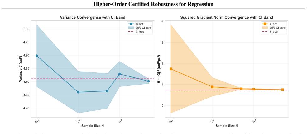
- Appendix J.2 convergence plots are useful; consider moving a single-panel summary of radius vs N into the main text so readers see that n=5k–10k is the operating regime for the reported claims.
Circularity Check
No circularity: certificates are solutions of an explicitly posed variational problem; empirical radii are independent measurements against PGD and α-smoothing.
full rationale
The derivation chain is self-contained and non-circular. The paper defines the smoothed regressor g, poses the nested max over perturbations and base functions consistent with observed moments (variance C, gradient G, mean E, bounds M), and solves it via calculus of variations / dual optimization (Props. 5.1–5.3, Cor. 5.4, Thm. 5.5 / H.1, Cor. 5.6, Algs. 1–4). The certified radius is the largest R with Δ_max(R)≤ε; that quantity is not defined in terms of the empirical comparison it later reports. Estimation of C and ∥G∥ uses standard U-statistics with asymptotic CIs (Sec. 6, App. I); those estimates are inputs to the certificate, not fitted parameters re-labeled as predictions of the same data. Related-work citations (Cohen, Levine, Mohapatra, Rekavandi) supply background, not a load-bearing uniqueness theorem by the present authors. The MNIST/UTKFace numbers (mean radius 0.210 vs 0.120, etc.) are empirical measurements of the resulting certificates against independent baselines and PGD attacks, not quantities forced by construction. Finite-sample coverage of the asymptotic CIs is a soundness limitation (as the paper itself notes), not circularity. Score 0; steps empty.
Assumptions & free parameters
free parameters (4)
- smoothing noise σ
- output tolerance ϵ
- failure probability α / success probability P
- Monte-Carlo sample size N
assumptions (3)
- standard math Base function f is square-integrable under the Gaussian measure so that Stein’s lemma applies and Var(f) ≥ σ^{2}∥G∥^{2}.
- domain assumption U-statistic estimators of variance and squared gradient norm are asymptotically normal, justifying the z-based confidence intervals used for certification.
- domain assumption The adversary is restricted to ℓ_{2}-bounded perturbations of the input.
Cite this review
Pith. "Pith review of Higher-Order Certified Robustness for Regression." pith.science (2026). https://pith.science/paper/BPKVMJUS
@misc{pith2026260705536,
  author       = {Pith},
  title        = {Pith review of: Higher-Order Certified Robustness for Regression},
  year         = {2026},
  howpublished = {\url{https://pith.science/paper/BPKVMJUS}},
  note         = {Machine review of arXiv:2607.05536}
}
read the original abstract
Randomized smoothing has emerged as a scalable technique for certifying the adversarial robustness of classifiers. However, its application to regression remains under-explored and faces unique challenges. Existing regression certificates rely on probabilistic acceptance regions and fail to exploit the local geometry of the function. In this work, we present a novel framework for certified robust regression that addresses these limitations. We derive a prediction-centered certificate that guarantees the stability of the smoothed model's prediction and ensures practical computability at test time. We investigate several alternatives for constructing these certificates by explicitly incorporating means, variances, and gradients. In particular, we demonstrate on the MNIST rotation task that utilizing gradient information yields significantly tighter robustness certificates compared to the current state-of-the-art, alpha-smoothing.
Figures


Figures from the paper (3 more)


Reference graph
Works this paper leans on
-
[1]
functional derivative
Equality in the Cauchy-Schwarz inequality holds if and only if f(x) is linearly related to Y almost everywhere. That is, f(x)−E[f(x)] = aY=aG ⊤(x−z)for some constanta. Plug the affine form into the gradient constraint. E[f(x)e] =E aG⊤e+E[f] e =aE (G⊤e)e +E[f]E[e]|{z} 0 Matching the gradient constraint, and givenE[ee ⊤] =σ 2I, we havea= 1. C. Our Problem a...
-
[2]
The objective is unchanged:∆(δ;f) = ∆(δ; ˜f)
-
[3]
The moment constraints transform to:E pz[ ˜f] = 0,E pz[ ˜f 2] = Varpz(f), and∇ zEpz[ ˜f] =∇ zEpz[f]
-
[4]
k pz+δ(x) pz(x) −1 2# =k 2Epz
The box constraint transforms to a shifted interval: ˜f(x)∈[−M−E, M−E]. Therefore, in the bounded setting, specifying the mean E is equivalent to specifying the location of the feasible box for the centered function. Proof. Points 1 and 2 follow immediately from the linearity of expectation and differentiation, identical to the logic in Lemma D.1. For poi...
-
[5]
Solving forµyields: µ=δ− σ2 k G.(20)
Solving for µ (Gradient Constraint):We substitute the general form f ∗(x)−g(z) =k(A−µ ⊤B) into the gradient constraintE[f ∗B] =G: G=E pz[(g(z) +k(A−µ ⊤B))B] =k Epz[AB]−E pz[BB ⊤]µ .(19) Applying Lemma F.1 (Items 1 and 2) to (19): G=k δ σ2 − 1 σ2 Iµ . Solving forµyields: µ=δ− σ2 k G.(20)
-
[6]
bang-bang
Solving fork(Variance Constraint):We substitute the form off ∗ into the variance constraintE[(f ∗ −g) 2] =C: C=k 2Epz (A−µ ⊤B)2 =k 2 Epz[A2]−2µ ⊤Epz[AB] +µ ⊤Epz[BB ⊤]µ .(21) 20 Higher-Order Certified Robustness for Regression Using Lemma F.1 in (21) results in: C=k 2(e ∥δ∥2 σ2 −1) + k2 σ2 µ⊤(µ−2δ). Substitutingµ−2δ=−(δ+ σ2 k G)from (20): µ⊤(µ−2δ) = δ− σ2 ...
-
[7]
The adversary can construct a step function (Neyman-Pearson solution) using only the values {−M, M} that satisfies the variance constraint trivially
The High-Variance Regime (C≥M 2 −E 2):The variance constraint is redundant. The adversary can construct a step function (Neyman-Pearson solution) using only the values {−M, M} that satisfies the variance constraint trivially. This reduces to the standard bounded certification problem (e.g., Cohen et al. (2019), Levine et al. (2020))
2019
-
[8]
The adversary is precluded from using a simple step function and must construct a solution that transitions smoothly or is clipped to satisfy the stricter variance budget
The Low-Variance Regime (C < M 2 −E 2):The variance constraint is strictly tighter than the natural bound imposed by M. The adversary is precluded from using a simple step function and must construct a solution that transitions smoothly or is clipped to satisfy the stricter variance budget. In the context of robust regression, we are specifically interest...
Show all 15 references
-
[9]
Stationarity Condition Taking the functional derivative ofL with respect to ϕ(t) and setting it to zero gives the necessary condition for the optimal solutionϕ ∗: δL δϕ(t) ϕ∗ = (w(t)−2λ(ϕ ∗(t)−E)−µ−η 1(t) +η 2(t))p 0(t) = 0 Rearranging forϕ ∗(t): 2λ(ϕ∗(t)−E) =w(t)−µ−η 1(t) +η 2(t)(28)
-
[10]
smoothed
KKT Conditions Forϕ ∗(t)to be optimal, it must satisfy: 24 Higher-Order Certified Robustness for Regression •Primal Feasibility:−M≤ϕ ∗(t)≤M. •Dual Feasibility:λ≥0,η 1(t)≥0, andη 2(t)≥0. •Complementary Slackness: λ(E[(ϕ∗ −E) 2]−C) = 0, η 1(t)(ϕ∗(t)−M) = 0, η 2(t)(−ϕ∗(t)−M) = 0 ...
-
[11]
The variance constraint is inactive (i.e.,λ= 0)
-
[12]
Bang-Bang
The optimal functionϕ ∗(t)is a Bang-Bang function (taking values in{−M−E, M−E}almost everywhere). Proof.LetLbe the Lagrangian of the problem. The pointwise maximization with respect toϕ(t)takes the form: ϕ∗(t) = arg max z∈[−M−E,M−E] z·L(t)−λz 2 whereL(t)is the effective linear...
-
[13]
Rearranging forϕ ∗(t): 2λϕ∗(t) =w(t)−µt−ν−η 1(t) +η 2(t)(41)
Stationarity Condition Taking the functional derivative ofL with respect to ϕ(t) and setting it to zero gives the necessary condition for the optimal solutionϕ ∗: δL δϕ(t) ϕ∗ = (w(t)−2λϕ ∗(t)−µt−ν−η 1(t) +η 2(t))p 0(t) = 0 Sincep 0(t)>0everywhere, the term in brackets must van...
-
[14]
•Dual Feasibility:λ≥0,η 1(t)≥0, andη 2(t)≥0
KKT Conditions Forϕ ∗(t)to be optimal, it must satisfy the Karush-Kuhn-Tucker conditions for allt: •Primal Feasibility:M lower ≤ϕ ∗(t)≤M upper. •Dual Feasibility:λ≥0,η 1(t)≥0, andη 2(t)≥0. •Complementary Slackness: λ(E[ϕ2]−C) = 0, η 1(t)(ϕ∗(t)−M upper) = 0, η 2(t)(−ϕ∗(t) +M lo...
-
[15]
edge cases
Variance (C):We calculate a two-sided interval [Clow, Chigh] and utilize the conservative upper bound Chigh. Due to the two-sided construction, the probability that the true variance exceeds this bound is at most α/4 (half of the α/2 budget). 2.Gradient Norm (∥G∥ 2):We calcula...
1992
Reviewed July 11, 2026 · model on record in the stance chip above.
Discussion (0). Sign in to comment.