REVIEW 2 major objections 6 minor 23 references
On the capacitance gradient description in Heterodyne Kelvin Probe Force Microscopy
T0 review · 2 major / 6 minor · reviewed 2026-08-02 · deepseek-v4-flash
Pith's one-line read A non-truncated Taylor expansion of the capacitance gradient exactly captures heterodyne KPFM spectral components at any oscillation amplitude.
desk verdict A rigorous Taylor-series framework for KPFM capacitance gradients that replaces the small-amplitude approximation, with a real caveat about the bimodal exactness claim. read the letter →
The pith
A machine-rendered reading of the paper's core claim, the machinery that carries it, and where it could break.
The reading
What carries the argument
The Hudlet-based capacitance-gradient model, split into cantilever, cone, and apex contributions, each a linear combination of functions 1/(z+ξ) and ln(z+a). The convergence proof maps the trajectory to a real variable x = δz/zc and shows |x| < 1 ≤ β, where β is the distance to the nearest singularity of these elementary functions, so the Taylor series converges term-by-term. The effective coefficients K0, K1, K2 (Eqs. 39–40) then carry the argument: they are infinite sums of higher-order CG derivatives with amplitude-weighted combinatorial factors, and the order-truncation regime criterion (comparing significance ratios ri,q against a threshold τ) decides when the leading first-order term s
What would settle it
Measure the ωmod sideband amplitude in a heterodyne experiment with a well-characterized sample while sweeping z1,0 over a range where K1 and C'' differ by more than a few percent; a deviation from the predicted K1 scaling that cannot be explained by the Hudlet geometry would falsify the model.
Extended reading notes
Core claim
The central claim is that the capacitance gradient C'(z(t)) along a sinusoidal tip trajectory can be represented exactly by its non-truncated Taylor series about the average tip–surface distance zc, provided the tip never touches the surface (zmin > 0). For the Hudlet-based model, the proof relies on the capacitance gradient being a linear combination of rational and logarithmic functions whose nearest singularities lie beyond the sampled distance range; hence the series converges regardless of oscillation amplitude. The static, ω1, and ω2 spectral components are then given exactly by the coefficients K0, K1, K2, which are infinite sums of higher-order spatial derivatives weighted by amplitu
Load-bearing premise
The capacitance and its gradient depend only on the instantaneous tip–surface distance, not on how fast the tip moves or on the bias-modulation frequency; if this quasi-static description fails, the position-only Taylor expansion no longer describes the actual electrostatic force.
Editorial extensions
If this is right
- Open-loop amplitude-modulation heterodyne KPFM can be modeled at arbitrary first-eigenmode amplitude by replacing C''(zc) with K1(zc), removing the vague small-amplitude restriction.
- The second-eigenmode coefficient K2 enters higher-order truncation regimes earlier than K1, making second-mode amplitude and phase observables more sensitive to short-range capacitance nonlinearity.
- Taylor-based coefficients converge to Fourier coefficients with exponentially decreasing error as truncation order increases, giving practical stopping rules for numerical simulation.
- The framework extends to incommensurate bimodal frequencies, where no finite Fourier super-period exists, because the Taylor representation is frequency-agnostic.
- The static coefficient K0 provides an exact expression for the DC electrostatic-force channel, which matters for interpreting force offsets in Kelvin probe measurements.
Reading between the lines
- If the quasi-static assumption breaks down, for instance due to dielectric relaxation in the sample at the bias-modulation frequency, the position-only Taylor expansion would no longer describe the actual force; discrepancies between K1-based predictions and measured sidebands could serve as a diagnostic for such rate-dependent capacitance.
- The same Taylor–Fourier machinery could be applied to other oscillating-probe observables that are nonlinear functions of tip–sample distance, such as van der Waals force gradients or microwave impedance, yielding analogous effective coefficients and truncation criteria.
- Because K2 is more sensitive to higher-order derivatives, deliberately tuning z1,0 and z2,0 into the higher-order regime could enhance contrast to subsurface or short-range dielectric variations, turning the small-amplitude approximation's failure into a useful measurement channel.
Signed reviews
Editorial analysis
A structured set of objections, weighed in public.
Referee Report
Summary. The paper develops a non-truncated Taylor-series description of the tip–sample capacitance gradient (CG) in heterodyne KPFM, for both monomodal and bimodal cantilever motion. It proves convergence of the Taylor expansion for a Hudlet-based CG model under the physically admissible condition zmin > 0, derives closed-form expressions for the effective CG coefficients K0, K1, K2 that govern the static, first-eigenmode, and second-eigenmode spectral components, and introduces order-truncation regimes (OTRs) with a term-significance criterion. Numerical simulations validate the convergence of Taylor-based coefficients to Fourier coefficients and map the OTRs in the (zc, z1,0) plane.
Significance. If the claims hold, the paper provides a rigorous replacement for the conventional first-order Taylor approximation, with explicit convergence guarantees and quantitative truncation criteria. The convergence proof for the elementary functions 1/(z+ξ) and ln(z+a) is clean and correct, and the closed-form coefficient expressions (Eqs. 25 and 40) are valuable for analyzing heterodyne KPFM observables. The numerical validation is thorough and reproducible from the stated parameters. The main caveat is the treatment of frequency commensurability, which requires qualification in the abstract and conclusions.
major comments (2)
- [Sec. II.C.2, Eqs. (39)–(41)] The identification of the effective coefficients with Fourier coefficients, Xp1 = K1 z1,0 and Xp2 = K2 z2,0, is stated without qualification, but it is exact only for incommensurate frequencies. For commensurate frequencies, integer combinations m1ω1 + m2ω2 can coincide with ω1 or ω2. For the paper's own ratio f1=10fs, f2=63fs, the first extra contribution to the ω1 component appears at Taylor order n = |1−63k| + 10k = 72 (k=1), and to the ω2 component at n=74. Thus for a non-truncated TSE, Eqs. (41b)–(41c) are not exact for commensurate trajectories; they hold only below the first coincidence order. The main text concedes this only in the sentence about the 'Taylor-order range considered here' and in SI Sec. III.G.2, while the abstract and conclusion present the coefficients as exact without this restriction. Since the abstract's claim of a 'rigorous spectral description' and 'effective
- [Sec. II.C.1] The text states that the framework 'applies to integer-multiple, commensurate, and incommensurate frequency relationships,' but the compact formulas presented in Sec. II.C.2 are derived only for incommensurate frequencies. The general commensurate case is not worked out in the main text; the SI only notes the absence of extra contributions for n ≤ 30. This is misleading: a reader cannot infer the validity range from the main text alone. I recommend either presenting the general coincidence-order condition in the main text or clearly marking Eqs. (39)–(40) as valid for incommensurate frequencies and for commensurate frequencies only below the first coincidence order.
minor comments (6)
- [Abstract and Conclusion] The abstract and conclusion should carry the same caveat about commensurate frequencies as the body text. As written, they assert general exactness that is not warranted for all frequency relationships.
- [Eq. (30)] The OTR order ℓ* is defined as the maximum q with ri,q ≥ τ. If the significance ratios are non-monotonic, the 'highest' significant order may not form a contiguous regime. Please clarify whether monotonic decay is assumed or whether the definition should be interpreted as a set of significant orders.
- [Sec. II.C.2, text before Eq. (40)] The sentence 'The compact expressions derived for incommensurate frequencies are used here' is placed after Eq. (39). It would be clearer to state this before presenting the formulas and to specify that the numerical validation uses n ≤ 30, where the extra commensurate terms are absent.
- [Fig. 10] The color map uses a single hue gradient for HOTR-2 through HOTR->5; distinguishing the boundaries would be easier with a discrete color bar and explicit labels for each regime.
- [Author list] The name 'Benjamin Gr´evin' contains a formatting artifact (the accent appears as a combining character). Please ensure the typesetting is correct.
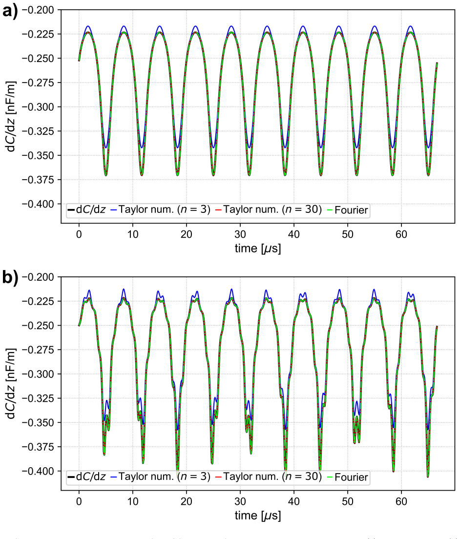
- [Sec. III.B.4] The sentence 'The static, f1, and f2 components retained in the Taylor-Fourier comparison remain clearly identifiable' is correct, but it would help to state explicitly that the numerical projection in Eq. (54) captures all components at f1 and f2, including any high-order commensurate terms, which is why the comparison is valid for n ≤ 30.
Circularity Check
No significant circularity: the Taylor–Fourier coefficient derivation is self-contained; companion-manuscript self-citation is downstream and not load-bearing.
full rationale
The central derivation starts from the non-truncated Taylor series Eq. (8) of the Hudlet-based CG, proves convergence in Sec. II A 3 from the elementary functions h1 and h2 under the admissible trajectory condition zmin > 0, and obtains the effective coefficients K0, K1, K2 in Eqs. (39)–(40) by binomial expansion and frequency selection. The numerical section III.B.6 projects the exact CG signal from the same Hudlet model onto static, f1, and f2 Fourier components (Eqs. (54)–(57)) and compares those projections with the Taylor-based coefficients; this is an internal consistency check of the mathematics, not a fit of parameters to data. No parameter is tuned to force agreement with a target, and no “prediction” is constructed from a fitted input. The only self-citation, the companion manuscript [16], is invoked for downstream force components, observables, and experimental heterodyne effects, not for Eqs. (39)–(40) or the convergence proof; hence it is not load-bearing. The main text itself limits the compact bimodal expressions to incommensurate frequencies and to the Taylor-order range considered, with commensurability-induced contributions absent over that range (Sec. III.G.2 of the SI), so the commensurability caveat is an explicit scope restriction rather than a hidden circular reduction. The paper is self-contained against the Hudlet model and internally consistent; no circular step is exhibited.
Assumptions & free parameters
free parameters (1)
- OTR significance threshold tau =
1e-2
assumptions (5)
- domain assumption The tip-surface CG is quasi-static: C(1)(z(t)) depends only on the instantaneous distance z(t), with no frequency- or history-dependent response.
- domain assumption The CG is described by the Hudlet-based model Eq. (9), a linear combination of 1/(z+xi) and ln(z+a) with the given geometric parameters.
- domain assumption The cantilever trajectory is a prescribed superposition of sinusoidal eigenmode displacements (Eqs. (3), (33)), and the motion is not modified by the electrostatic force (open-loop).
- domain assumption Physically admissible trajectories satisfy zmin = zc - zdyn > 0, so the tip never reaches the surface.
- standard math For periodic analytic trajectories, the function C(1)(z(t)) admits both a convergent Taylor series in delta z and a Fourier series in time, and the two can be equated term-wise via binomial expansion.
Cite this review
Pith. "Pith review of On the capacitance gradient description in Heterodyne Kelvin Probe Force Microscopy." pith.science (2026). https://pith.science/paper/SDYP3CMM
@misc{pith2026260706161,
  author       = {Pith},
  title        = {Pith review of: On the capacitance gradient description in Heterodyne Kelvin Probe Force Microscopy},
  year         = {2026},
  howpublished = {\url{https://pith.science/paper/SDYP3CMM}},
  note         = {Machine review of arXiv:2607.06161}
}
read the original abstract
Kelvin probe force microscopy (KPFM) probes local surface-potential variations through the electrostatic force between a conductive tip and a surface, which depends on the potential difference and the tip-surface capacitance gradient (CG). In heterodyne KPFM, the oscillating tip is usually treated by combining a bias-modulated electric field with a first-order truncated Taylor-series expansion of the CG. Although convenient, this treatment is limited to a poorly defined small-amplitude regime and leaves the convergence of the series unresolved. Here, we establish a rigorous spectral description of the CG dynamics and of the resulting electrostatic force beyond this approximation. We formulate a non-truncated Taylor-series description of the CG and prove its convergence for a realistic Hudlet-based capacitance model in both monomodal and bimodal motion. In the monomodal case, we show the equivalence between Fourier-series and Taylor-series descriptions, derive explicit expressions for the dominant Fourier coefficients, and introduce order-truncation criteria that replace the usual qualitative notion of a small-amplitude regime. We then extend the formalism to bimodal motion and derive the effective CG coefficients governing the static, first-eigenmode, and second-eigenmode components of the electrostatic interaction. Numerical simulations confirm the convergence of the Taylor-based coefficients toward the Fourier coefficients and support the truncation-regime hierarchy in both configurations. This work establishes the formal basis for describing electrostatic force components and AFM observables in open-loop heterodyne experiments and provides a general framework for CG dynamics in multimode force microscopy involving nonlinear electromechanical coupling and frequency conversion.
Figures


Figures from the paper (17 more)




Reference graph
Works this paper leans on
-
[1]
Melitz, J
W. Melitz, J. Shen, A. Kummel, and S. Lee, Surf. Sci. Rep.66, 1 (2011)
2011
-
[2]
Sadewasser and T
S. Sadewasser and T. Glatzel, eds.,Kelvin Probe Force Microscopy: Measuring and Compen- sating Electrostatic Forces, Vol. 48 (Springer, 2012)
2012
-
[3]
Sadewasser and T
S. Sadewasser and T. Glatzel, eds.,Kelvin Probe Force Microscopy: From Single Charge Detection to Device Characterization, Vol. 65 (Springer, 2018)
2018
-
[4]
Lord Kelvin (William Thomson), Philosophical Magazine Series 546, 82 (1898)
-
[5]
Zisman, Rev
W. Zisman, Rev. Sci. Instrum.3, 367 (1932)
1932
-
[6]
(1a), the term ( VDC −V cpd) assumes that the bias is applied to the sample while the tip is grounded
In Eq. (1a), the term ( VDC −V cpd) assumes that the bias is applied to the sample while the tip is grounded. It must be recast as ( VDC + Vcpd) when the opposite bias convention is used
-
[7]
Sugawara, L
Y. Sugawara, L. Kou, Z. Ma, T. Kamijo, Y. Naitoh, and Y. J. Li, Appl. Phys. Lett.100, 223104 (2012)
2012
-
[8]
Bonnell, D
D. Bonnell, D. Basov, M. Bode, U. Diebold, S. Kalinin, V. Madhavan, L. Novotny, M. Salmeron, U. Schwarz, and P. Weiss, Rev. Mod. Phys.84, 1343 (2012)
2012
Show all 23 references
-
[9]
Borgani, D
R. Borgani, D. Forchheimer, J. Bergqvist, P.-A. Thor´ en, O. Ingan¨ as, and D. Haviland, Appl. Phys. Lett.105, 143113 (2014)
2014
-
[10]
A. Axt, I. Hermes, V. Bergmann, N. Tausendpfund, and S. Weber, Beilstein J. Nanotechnol.9, 1809 (2018)
2018
-
[11]
Garrett, M
J. Garrett, M. Leite, and J. Munday, ACS Appl. Mater. Interfaces10, 28850 (2018)
2018
-
[12]
Dwyer, L
R. Dwyer, L. Harrell, and J. Marohn, Phys. Rev. Applied11, 064020 (2019)
2019
-
[13]
Borgani and D
R. Borgani and D. Haviland, Rev. Sci. Instrum.90, 013705 (2019)
2019
-
[14]
Garrett, D
J. Garrett, D. Somers, K. Sendgikoski, and J. Munday, Phys. Rev. A100, 022508 (2019)
2019
-
[15]
Gr´ evin, F
B. Gr´ evin, F. Husainy, D. Aldakov, and C. Auma ˆ ıtre, Beilstein J. Nanotechnol.14, 1068 (2023)
2023
-
[16]
Valloire, S
H. Valloire, S. Clair, C. Loppacher, L. Nony, and B. Gr´ evin, Inverse heterodyne effect in bimodal Kelvin probe force microscopy, submitted to APS Open Sci. (2026)
2026
-
[17]
Jahng, B
J. Jahng, B. Kim, E. Lee, and E. Potma, Phys. Rev. B94, 195407 (2016)
2016
-
[18]
Hudlet, M
S. Hudlet, M. S. Jean, C. Guthmann, and J. Berger, Eur. Phys. J. B2, 5 (1998)
1998
-
[19]
Rodr ´ ıguez and R
T. Rodr ´ ıguez and R. Garc ´ ıa, Appl. Phys. Lett.84, 449 (2004)
2004
-
[20]
Lozano and R
J. Lozano and R. Garcia, Phys. Rev. Lett.100, 076102 (2008). 37
2008
-
[21]
Lozano and R
J. Lozano and R. Garcia, Phys. Rev. B79, 014110 (2009)
2009
-
[22]
Kawai, T
S. Kawai, T. Glatzel, S. Koch, B. Such, A. Baratoff, and E. Meyer, Phys. Rev. Lett.103, 220801 (2009)
2009
-
[23]
num” and “ana
C.-Y. Lai, V. Barcons, S. Santos, and M. Chiesa, J. Appl. Phys.118, 044905 (2015). 38 FIGURES FIG. 1:Geometry of the problem. Schematic representation of the cantilever oscillatory motion above the sample surface in the monomodal and bimodal regimes. The blue solid curve repre...
2015
Reviewed August 2, 2026 · model on record in the stance chip above.
Discussion (0). Continue with ORCID to comment.