REVIEW 2 major objections 8 minor 74 references
Learning Turbulence Closures with Physics-Informed Neural Networks for the Rayleigh-Taylor Transition to Turbulence
T0 review · 2 major / 8 minor · reviewed 2026-07-09 · glm-5.2
Pith's one-line read Neural networks teach a turbulence model the missing physics of transition
desk verdict Solid framework for RT transition closures; the analytical correction works but its feedback stability under standalone integration is untested. read the letter →
The pith
A machine-rendered reading of the paper's core claim, the machinery that carries it, and where it could break.
The reading
What carries the argument
The central machinery is a three-stage pipeline: (1) a physics-informed neural network (PINN) that solves the RANS equations while simultaneously calibrating model coefficients against DNS data; (2) an augmented PINN with a separate correction network that disentangles parametric errors (wrong coefficients) from structural errors (missing physics) by penalizing the correction terms so that calibration absorbs what it can and the correction absorbs the rest; (3) symbolic regression that re-expresses the neural correction as an explicit analytical function of two physically motivated variables—the Froude number Fr and the directed-to-total kinetic energy ratio k_d/k—yielding a portable, human-
What would settle it
Integrate the corrected model on DNS trajectories outside the training set and outside the restricted parameter range (R < 14 or D > 2). If the corrected model fails to reproduce the dissipation peak or the self-similar growth rate in these regimes, the two-variable formula is insufficient and additional dependencies are needed.
Extended reading notes
Core claim
The structural error of the k-epsilon-b model during Rayleigh-Taylor transition is localized in the dissipation equation, and can be corrected by making the production coefficient C_epsilon_0 depend on the Froude number and the directed-to-total kinetic energy ratio via the explicit formula of Eq. (11). This single modification, derived by symbolic regression on neural-network-inferred corrections, enables the baseline model to capture the enstrophy blow-up and dissipation peak during transition while preserving the correct asymptotic self-similar growth rate. A notable side effect is that the concentration variance b, passive in the original model, becomes dynamically coupled to k and epsil
Load-bearing premise
The directed kinetic energy k_d, defined as half the squared concentration flux divided by the concentration variance and derived from a first-gradient closure, is assumed to be an adequate single proxy for the spectral imbalance between buoyancy-driven energy transfer and small-scale dissipation during transition. If the transition dynamics depend on additional spectral information not captured by this ratio, the analytical correction will be incomplete.
Editorial extensions
If this is right
- The corrected k-epsilon-b model can be directly implemented in production simulation codes for inertial confinement fusion and astrophysical mixing, improving transition predictions without requiring on-the-fly neural network inference.
- The methodology—PINN-based error disentanglement followed by symbolic regression—provides a general recipe for extracting interpretable corrections from any RANS closure, applicable to other transitional or non-equilibrium flows beyond Rayleigh-Taylor.
- The activation of the concentration variance b as a dynamically coupled variable suggests that passive scalar transport equations in other buoyancy-driven flows may harbor hidden structural couplings that similar analysis could reveal.
- The finding that one coefficient (C_epsilon_0) carries the dominant structural error identifies the dissipation production term as the primary locus of missing physics in transitional Rayleigh-Taylor, guiding future model development even without data-driven methods.
Reading between the lines
- The restriction of the analytical correction to inertial trajectories (R >= 14, D <= 2) implies that very low Reynolds number or highly diffusive initial conditions may involve additional spectral physics not captured by the two-variable formula; extending to the full parameter space would likely require an explicit Reynolds-number dependence.
- The directed-energy proxy k_d defined via the first-gradient closure may lose accuracy in regimes where the gradient-diffusion hypothesis itself breaks down—such as strongly non-local transport—suggesting that a second-order closure for the scalar flux could improve the fidelity of the correction without adding much complexity.
- If the methodology were applied to Richtmyer-Meshkov instability (impulsive acceleration rather than sustained), the structural error might localize in a different equation or require a different set of flow indicators, since the spectral imbalance between buoyancy and dissipation has a different temporal structure.
Editorial analysis
A structured set of objections, weighed in public.
Referee Report
Summary. This manuscript addresses a problem of practical importance: the failure of standard RANS k-epsilon-b closures to capture the transition to turbulence in Rayleigh-Taylor (RT) mixing, specifically the dissipation peak associated with enstrophy blow-up. The authors embed the turbulence model within a physics-informed neural network (PINN), calibrate its coefficients against an extensive DNS database (484 simulations), and use corrective neural-network terms to disentangle parametric from structural model errors. The key structural correction is localized to the dissipation-production coefficient C_{epsilon0}, which is then re-expressed via symbolic regression as an analytical function of the Froude number and a directed-to-total kinetic energy ratio. The resulting corrected model is tested on held-out trajectories and shown to capture both the transition and the correct self-similar growth rate. The methodology is well-motivated, the use of an extensive DNS database is a clear strength, and the final analytical correction is interpretable and deployable in production codes.
Significance. The paper makes a solid contribution to data-driven turbulence closure development. Its principal strengths are: (1) the use of a large, systematically parameterized DNS database (484 simulations) embedded in a PINN surrogate, providing a robust training and validation foundation; (2) a clear and physically motivated strategy for disentangling parametric from structural errors via penalized correction networks; (3) the derivation of a compact, interpretable analytical correction (Eq. 11) that can be directly implemented in existing RANS solvers without requiring neural-network inference at runtime; and (4) honest error reporting (Table V) that quantifies the degradation from the full PINN correction to the analytical surrogate. The framework is general and could be applied to other flow regimes. The work fits well within the scope of a fluid-dynamics journal.
major comments (2)
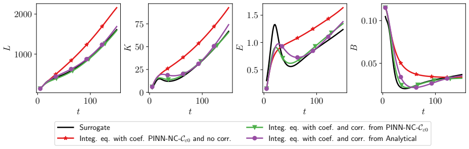
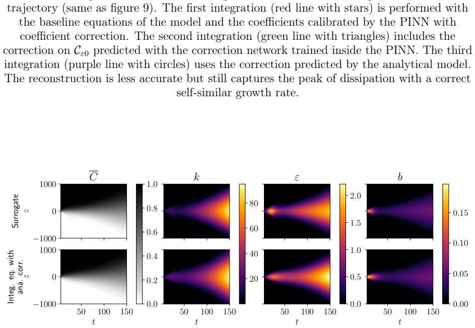
- Section IV, Eq. (11): The analytical correction for C_{epsilon0} is derived via symbolic regression applied to outputs of the PINN-NC-C_{epsilon0} network, whose inputs (partial_z C_hat, k_hat, epsilon_hat, b_hat) come from the PINN prediction network and closely match DNS. When the analytical model is integrated standalone (Figs. 12-14), Fr and k_d/k are computed from the k-epsilon-b model's own state variables, which inevitably drift from DNS during the transition phase. This creates a feedback loop: model errors in the state variables alter the correction, which in turn alters the state variables. Table V shows the analytical model's MRE on L is 6.35%, roughly 2x the PINN-NC-C_{epsilon0}'s 3.30% and 3x the PINN-C-f's 2.18%. The paper does not analyze whether this degradation is benign (self-stabilizing) or potentially pathological (small state errors amplifying through Eq. (11)'s form
- Section IV, Eq. (11) and Table V: The restriction of the analytical model's training and evaluation to 'inertial trajectories' (R >= 14, D <= 2) is stated but its implications are not fully discussed. How large is the excluded portion of the parameter space, and what happens when the analytical correction is applied outside this range? The authors note that 'seeking an analytical expression for the coefficient over the full dataset would require an additional dependence on the Reynolds number,' but they do not quantify the failure mode. Since the stated goal is improving RT transition predictions broadly, the practical utility of a correction valid only for a subset of initial conditions should be clarified.
minor comments (8)
- The notation alternates between k-epsilon-b and k-epsilon-b without consistent hyphenation. Standardizing throughout would improve readability.
- Fig. 8 is information-dense; the four columns of decomposition terms (diffusion, production, dissipation, correction) are difficult to distinguish at the scale shown. Consider enlarging or separating the four quantities.
- Table I: the caption notes that Bayesian intervals are 'given at 95%' but the text says they represent standard deviation. This is contradictory; please clarify whether the intervals are 95% credible intervals or plus/minus one standard deviation.
- Section III.B.2: The text states 'the unusual notation gamma for the standard deviation is used to avoid any confusion with the sigmas already appearing in the model,' but gamma is also used for the penalty hyperparameter lambda_penalty in later sections. Using a different symbol would avoid potential confusion.
- Eq. (10): The definition of directed energy k_d = (1/2)(u_z c)^2 / b is introduced following [52], but the physical justification for this specific decomposition is brief. A sentence explaining why this ratio captures 'large-scale coherent structure energy' would aid readers unfamiliar with the reference.
- The abstract describes the corrected model as 'fully interpretable,' but Eq. (11) contains an exponent of 3.185 and several fitted constants. While the functional form is explicit, the claim of 'fully interpretable' could be softened to 'analytical' or 'physically motivated.'
- Appendix B.3.d: The choice of Softplus parameter beta is mentioned in Eq. (B10) but its value is not specified. Please state the value of beta used.
- Fig. 12: The three integrated solutions are visually difficult to distinguish in the printed version. Consider using more distinct line styles or a table of quantitative metrics at selected times to complement the figure.
Circularity Check
No significant circularity; the analytical correction is transparently a fit to PINN outputs, and standalone integration on held-out DNS trajectories is a genuine generalization test, not a self-fulfilling prediction.
full rationale
The paper's derivation chain is: (1) 484 DNS simulations → surrogate PINN model (verified against DNS); (2) surrogate → calibration of k-ε-b coefficients via regression, Bayesian MCMC, and PINN-C (standard calibration, with independent recovery of α_∞ ≈ 0.02 via Eq. 8); (3) PINN-C-f with corrective terms → disentangle parametric vs. structural errors (physical insight: structural error localizes in the dissipation equation); (4) PINN-NC-C_ε0 → re-express correction as a function of model state variables; (5) symbolic regression on PINN-NC-C_ε0 outputs → analytical formula Eq. (11) for C_ε0(Fr, k_d/k); (6) standalone integration of the analytical model → comparison against held-out DNS trajectories (Figs. 12–14, Tab. V). The paper is transparent that Eq. (11) is a fit: 'we apply symbolic regression to the coefficient represented by the corrective neural network in the PINN.' The standalone integration is a genuine generalization test because the model's own state variables (which drift from DNS during transition) feed back into the formula, creating a feedback loop that is not protected by the PINN's coupling to DNS-accurate data. The 2× error increase (3.30% → 6.35% MRE on L) is consistent with the formula being an approximation of the neural network, not with circularity. Self-citations exist ([14, 15] for the DNS database and surrogate, [52] for the directed energy definition), but these provide independently generated computational data and a physical ansatz, not theorems invoked to force the conclusion. The physical quantities Fr and k_d/k are independently motivated by Rayleigh-Taylor phenomenology. No step in the chain reduces to its own inputs by construction.
Assumptions & free parameters
free parameters (11)
- σ_c =
0.126
- σ_k =
0.106
- σ_ε =
0.195
- σ_b =
0.187
- C_ε0 =
1.358 (asymptotic)
- C_ε2 =
1.92
- C_χ =
0.934
- C_μ =
0.09
- λ_penalty =
10^-3
- Eq. (11) constants =
1.252, 0.113, 0.555, 0.397, 3.185, 0.625, 0.404
- C_ε0 clamping bounds =
[1, 4]
assumptions (5)
- domain assumption Boussinesq approximation: density variations are negligible except in the buoyancy term.
- domain assumption First-gradient closure for turbulent concentration flux: u_z c = -(ν_t/σ_c)∂_z C.
- ad hoc to paper Directed energy k_d = (1/2)(u_z c)^2/b adequately represents large-scale coherent energy.
- domain assumption Piecewise-linear C profile and parabolic k, ε, b profiles within the mixing zone.
- domain assumption ν = κ (kinematic viscosity equals diffusion coefficient).
invented entities (1)
-
Directed energy k_d
Cite this review
Pith. "Pith review of Learning Turbulence Closures with Physics-Informed Neural Networks for the Rayleigh-Taylor Transition to Turbulence." pith.science (2026). https://pith.science/paper/SBPQR2XL
@misc{pith2026260707020,
  author       = {Pith},
  title        = {Pith review of: Learning Turbulence Closures with Physics-Informed Neural Networks for the Rayleigh-Taylor Transition to Turbulence},
  year         = {2026},
  howpublished = {\url{https://pith.science/paper/SBPQR2XL}},
  note         = {Machine review of arXiv:2607.07020}
}
abstract
Reynolds-averaged Navier-Stokes (RANS) turbulence models are known to perform poorly in predicting the dynamics of Rayleigh-Taylor mixing when turbulence is not fully developed, particularly during the transition from an initially perturbed interface. In this work, we investigate the use of data-driven strategies to enhance a simple $k$-$\varepsilon$-$b$ model for this transitional regime. The turbulence model is first embedded within a surrogate physics-informed neural network (PINN), enabling the calibration of coefficients that account for parametric errors and the identification of corrective terms representing structural errors associated with missing physical processes. The learned corrections are then re-expressed onto the model state variables and relevant flow indicators, leading to explicit analytical modifications of the closure. The resulting fully interpretable corrected model is assessed against an extensive database of direct numerical simulations (DNS) of Rayleigh-Taylor flows. This framework enables improved predictions of the mixing-layer growth during the transition to turbulence.
Figures


Figures from the paper (16 more)




Reference graph
Works this paper leans on
-
[1]
and the calibration of RANS models including the Rayleigh–Taylor instability. These approaches offer the advantage of not requiring a dedicated RANS solver, as the RANS model can be incorporated directly into the loss function [35, 36]. Moreover, it has been demonstrated that, by augmenting PINNs with an additional neural network while enforcing the model...
work page 2000
-
[2]
This makes it possible to set the value ofCε2 to 1.92, as is commonly done in most RANS models [49]
Methodology The calibration of a RANS model can first be carried out on solutions of simplified turbulent flows, foremost among them the decay of homogeneous isotropic turbulence. This makes it possible to set the value ofCε2 to 1.92, as is commonly done in most RANS models [49]. Similarly we fix the coefficient setting the turbulent viscosity atCµ = 0.09...
-
[3]
Results The calibration results obtained on the Rayleigh–Taylor dataset, following the procedures detailed above, are reported in Table I. As can be seen, the calibrated coefficients obtained from the different approaches—regression, Bayesian calibration, and PINN-C 0D or 1D— are in good agreement. In particular, one first observes that calibrating the mo...
-
[4]
Linear regression To determine the appropriate coefficients, perhaps the most elementary approach is to apply a linear regression to the data using thek–ε–bequations. The data are restricted to the time intervalt∈[80,150], which corresponds to ana prioridomain of validity for the model, since the self-similar regime has already begun, although it is not y...
-
[5]
The idea for the calibration is similar to the one performed by Nadiga et al
Dynamics Bayesian calibration Thissectiondescribesthemethodusedtoperformabayesiancalibrationofthecoefficients using a Monte-Carlo Markov Chains (MCMC) [57] method. The idea for the calibration is similar to the one performed by Nadiga et al. [32]. The Bayes theorem [58] yields: P(β|q) = P(q|β)P(β) P(q) (B2) withP(β)the prior,P(β|q)the posterior andP(q|β)t...
-
[6]
27 0.13435 0.13440 0.13445 σc 0 10000 20000p
Calibration using physics informed neural-networks, PINN-C This section describes the procedure used to calibrate the coefficients with the PINNs. 27 0.13435 0.13440 0.13445 σc 0 10000 20000p. d. f. 0.00025 0.00050 0.00075 Cε0 +1.375 0 2000 4000 6000p. d. f. 0.925 0.926 Cχ 0 1000 2000p. d. f. Chain 1 Chain 2 Chain 3 Chain 4 FIG. 15: Posterior obtained wit...
work page 2000
-
[7]
Force corrections PINN-C-f This section describes the changes made to the calibration setup to introduce forces in the PINN in order to both calibrate and correct the model. a. Training setup The prediction network and the trainable weights associated with the coefficients are left unchanged, and a new neural network is added to predict the correction for...
-
[8]
Physics informed neural network with coefficient correction PINN-NC-Cε0 This section describes the modifications made to the initial PINN setup to introduce a model correction for theCε0 coefficient as presented in Fig. 10. a. Training setup As for the force correction, the prediction network is left unchanged. The formerly train- able coefficients are re...
Show all 74 references
-
[9]
J. W. S. Rayleigh, Proceedings of the London Mathematical Society6, 170 (1882)
-
[10]
G. I. Taylor, Proceedings of the Royal Society of London. Series A pp. 192–196 (1950)
1950
-
[11]
Zhou, Physics Reports720-722, 1 (2017), ISSN 0370-1573, rayleigh–Taylor and Richt- myer–Meshkov instability induced flow, turbulence, and mixing
Y. Zhou, Physics Reports720-722, 1 (2017), ISSN 0370-1573, rayleigh–Taylor and Richt- myer–Meshkov instability induced flow, turbulence, and mixing. I, URLhttps://www. sciencedirect.com/science/article/pii/S0370157317302958
2017
-
[12]
Zhou, Physics Reports723-725, 1 (2017), ISSN 0370-1573, rayleigh–Taylor and Richt- myer–Meshkov instability induced flow, turbulence, and mixing
Y. Zhou, Physics Reports723-725, 1 (2017), ISSN 0370-1573, rayleigh–Taylor and Richt- myer–Meshkov instability induced flow, turbulence, and mixing. II, URLhttps://www. sciencedirect.com/science/article/pii/S0370157317302958
2017
-
[13]
Lindl, Physics of Plasmas2, 3933 (1995), ISSN 1070-664X, 1089- 7674, URLhttps://pubs.aip.org/pop/article/2/11/3933/261855/ Development-of-the-indirect-drive-approach-to
J. Lindl, Physics of Plasmas2, 3933 (1995), ISSN 1070-664X, 1089- 7674, URLhttps://pubs.aip.org/pop/article/2/11/3933/261855/ Development-of-the-indirect-drive-approach-to
1995
-
[14]
Betti and O
R. Betti and O. A. Hurricane, Nature Physics12, 435 (2016), ISSN 1745-2481, URLhttps: //www.nature.com/articles/nphys3736
2016
-
[15]
B. A. Remington, H.-S. Park, D. T. Casey, R. M. Cavallo, D. S. Clark, C. M. Huntington, D. H. Kalantar, C. C. Kuranz, A. R. Miles, S. R. Nagel, et al., Proceedings of the National Academy of Sciences116, 18233 (2019), ISSN 0027-8424, 1091-6490, URLhttps://pnas. org/doi/10.1073...
2019 doi
-
[16]
Y. Zhou, J. D. Sadler, and O. A. Hurricane, Annual Review of Fluid Mechanics57, 197 (2025), ISSN 0066-4189, 1545-4479, URLhttps://www.annualreviews.org/content/journals/10. 1146/annurev-fluid-022824-110008
2025
-
[17]
D. H. Sharp, Physica D: Nonlinear Phenomena12, 3 (1984), ISSN 0167-2789, URLhttps: //www.sciencedirect.com/science/article/pii/0167278984905104
1984
-
[18]
Chandrasekhar,Hydrodynamic and hydromagnetic stability(Courier Corporation, 2013)
S. Chandrasekhar,Hydrodynamic and hydromagnetic stability(Courier Corporation, 2013)
2013
-
[19]
V. N. Goncharov, Physical Review Letters88, 134502 (2002), URLhttps://link.aps.org/ doi/10.1103/PhysRevLett.88.134502
2002 doi
-
[20]
A. W. Cook and P. E. Dimotakis, Journal of Fluid Mechanics443, 69 (2001). 40
2001
-
[21]
D. L. Youngs, Physica D: Nonlinear Phenomena12, 32 (1984)
1984
-
[22]
Thévenin, B.-J
S. Thévenin, B.-J. Gréa, G. Kluth, and B. Nadiga, Journal of Fluid Mechanics0, A1 (2025), URLhttps://doi.org/10.1017/jfm.2025.209
2025 doi
-
[23]
Thévenin and B.-J
S. Thévenin and B.-J. Gréa, Physica D: Nonlinear Phenomena483, 134947 (2025), ISSN 0167- 2789, URLhttps://www.sciencedirect.com/science/article/pii/S0167278925004245
2025
-
[24]
J. D. Ramshaw, Physical Review E58, 5834 (1998), ISSN 1063-651X, 1095-3787, URLhttps: //link.aps.org/doi/10.1103/PhysRevE.58.5834
1998 doi
-
[25]
Dimonte, Physics of Plasmas7, 2255 (2000), ISSN 1070-664X, 1089-7674, URLhttps://pubs.aip.org/pop/article/7/6/2255/103605/ Spanwise-homogeneous-buoyancy-drag-model-for
G. Dimonte, Physics of Plasmas7, 2255 (2000), ISSN 1070-664X, 1089-7674, URLhttps://pubs.aip.org/pop/article/7/6/2255/103605/ Spanwise-homogeneous-buoyancy-drag-model-for
2000
-
[26]
D. L. Youngs and B. Thornber, Physica D: Nonlinear Phenomena410, 132517 (2020), ISSN 0167-2789, URLhttps://www.sciencedirect.com/science/article/pii/ S0167278919307146
2020
-
[27]
Schilling, Physica D: Nonlinear Phenomena402, 132238 (2020)
O. Schilling, Physica D: Nonlinear Phenomena402, 132238 (2020)
2020
-
[28]
S. W. Haan, Physical Review A39, 5812 (1989), URLhttps://link.aps.org/doi/10.1103/ PhysRevA.39.5812
1989
-
[29]
S. W. Haan, Physics of Fluids B: Plasma Physics3, 2349 (1991), ISSN 0899-8221, URLhttps://pubs.aip.org/pfb/article/3/8/2349/812849/ Weakly-nonlinear-hydrodynamic-instabilities-in
1991
-
[30]
D. Ofer, U. Alon, D. Shvarts, R. L. McCrory, and C. P. Verdon, Physics of Plasmas3, 3073 (1996), ISSN 1070-664X, 1089-7674, URLhttps://pubs.aip.org/pop/article/3/8/3073/ 262868/Modal-model-for-the-nonlinear-multimode-Rayleigh
1996
-
[31]
Rollin and M
B. Rollin and M. J. Andrews, Journal of Turbulence14, 77 (2013), ISSN 1468-5248, URL http://www.tandfonline.com/doi/abs/10.1080/14685248.2013.790549
2013 doi
-
[32]
M.-J. Xiao, H. Qi, and Y.-S. Zhang, Journal of Fluid Mechanics1002, A4 (2025)
2025
-
[33]
H. Qi, Z. He, A. Xu, and Y. Zhang, Physica D: Nonlinear Phenomena483, 134975 (2025), ISSN 0167-2789, URLhttps://www.sciencedirect.com/science/article/pii/ S016727892500452X
2025
-
[34]
Duraisamy, G
K. Duraisamy, G. Iaccarino, and H. Xiao, Annual Review of Fluid Mechanics51, 357–377 (2019), ISSN 1545-4479, URLhttps://www.annualreviews.org/content/journals/10. 1146/annurev-fluid-010518-040547. 41
2019
-
[35]
Duraisamy, Phys
K. Duraisamy, Phys. Rev. Fluids6, 050504 (2021), URLhttps://link.aps.org/doi/10. 1103/PhysRevFluids.6.050504
2021
-
[36]
Xiao and P
H. Xiao and P. Cinnella, Progress in Aerospace Sciences108, 1–31 (2019), ISSN 0376-0421, URLhttps://www.sciencedirect.com/science/article/pii/S0376042118300952
2019
-
[37]
Boureima, V
I. Boureima, V. Gyrya, J. A. Saenz, S. Kurien, and M. Francois, Journal of Computational Physics457, 110924 (2022)
2022
-
[38]
J. M. Gimenez and F. Bre, Journal of Wind Engineering and Industrial Aerodynamics193, 103978 (2019), ISSN 0167-6105, URLhttps://www.sciencedirect.com/science/article/ pii/S0167610519305781
2019
-
[39]
Edeling, P
W. Edeling, P. Cinnella, R. Dwight, and H. Bijl, Journal of Computational Physics258, 73–94 (2014), ISSN 0021-9991, URLhttps://www.sciencedirect.com/science/article/ pii/S0021999113007031
2014
-
[40]
Nadiga, C
B. Nadiga, C. Jiang, and D. Livescu, Journal of Computational Physics394, 280 (2019)
2019
-
[41]
Raissi, P
M. Raissi, P. Perdikaris, and G. E. Karniadakis, Journal of Computational Physics (2019)
2019
-
[42]
Eivazi, M
H. Eivazi, M. Tahani, P. Schlatter, and R. Vinuesa, Physics of Fluids34(2022)
2022
-
[43]
Xiao, T.-C
M.-J. Xiao, T.-C. Yu, Y.-S. Zhang, and H. Yong, Computers & Fluids266, 106025 (2023)
2023
-
[44]
Zhang, K
Z. Zhang, K. Shukla, Z. Wang, A. Morales, T. Käufer, S. Salauddin, N. Walters, D. Barrett, K. Ahmed, M. S. Triantafyllou, et al., Journal of Fluid Mechanics1034, A16 (2026)
2026
-
[45]
Z. Zou, X. Meng, and G. E. Karniadakis, Journal of Computational Physics505, 112918 (2024), ISSN 0021-9991, URLhttps://www.sciencedirect.com/science/article/pii/ S0021999124001670
2024
-
[46]
Patel, V
Y. Patel, V. Mons, O. Marquet, and G. Rigas, Phys. Rev. Fluids9, 034605 (2024), URL https://link.aps.org/doi/10.1103/PhysRevFluids.9.034605
2024 doi
-
[47]
Kenjereš and K
S. Kenjereš and K. Hanjalić, Phys. Rev. E62, 7987 (2000), URLhttps://link.aps.org/ doi/10.1103/PhysRevE.62.7987
2000 doi
-
[48]
Schilling and N
O. Schilling and N. J. Mueschke, Phys. Rev. E96, 063111 (2017), URLhttps://link.aps. org/doi/10.1103/PhysRevE.96.063111
2017 doi
-
[49]
Thévenin, B.-J
S. Thévenin, B.-J. Gréa, G. Kluth, and A. Briard,Database of direct numerical simu- lations of Rayleigh-Taylor turbulence at low density contrast: 0D volume-averaged quan- tities(2025), URLhttps://entrepot.recherche.data.gouv.fr/citation?persistentId= doi:10.57745/VTM1PN. 42
2025 doi
-
[50]
Gréa and A
B.-J. Gréa and A. Briard, Phys. Rev. Fluids4, 064608 (2019), URLhttps://link.aps.org/ doi/10.1103/PhysRevFluids.4.064608
2019 doi
-
[51]
Briard, L
A. Briard, L. Gostiaux, and B.-J. Gréa, Journal of Fluid Mechanics883, A57 (2020)
2020
-
[52]
Briard, B.-J
A. Briard, B.-J. Grea, L. Oteski, O. Soulard, J. Griffond, S. Thevenin, and L. Danaila, Com- puters & Fluids p. 106741 (2025)
2025
-
[53]
Briard, B.-J
A. Briard, B.-J. Gréa, and O. Soulard, Journal of Fluid Mechanics1023, A20 (2025)
2025
-
[54]
Dimonte, D
G. Dimonte, D. L. Youngs, A. Dimits, S. Weber, M. Marinak, S. Wunsch, C. Garasi, A. Robinson, M. J. Andrews, P. Ramaprabhu, et al., Phys. Fluids16, 1668 (2004), URL http://scitation.aip.org/content/aip/journal/pof2/16/5/10.1063/1.1688328
2004 doi
-
[55]
M. J. Andrews and D. B. Spalding, Physics of Fluids A: Fluid Dynamics2, 922 (1990), http://dx.doi.org/10.1063/1.857652, URLhttp://dx.doi.org/10.1063/1.857652
1990 doi
-
[56]
Hanjalić, Annual Review of Fluid Mechanics34, 321–347 (2002), ISSN 1545- 4479, URLhttps://www.annualreviews.org/content/journals/10.1146/annurev.fluid
K. Hanjalić, Annual Review of Fluid Mechanics34, 321–347 (2002), ISSN 1545- 4479, URLhttps://www.annualreviews.org/content/journals/10.1146/annurev.fluid. 34.082801.161035
2002 doi
-
[57]
Meldi and P
M. Meldi and P. Sagaut, Journal of Fluid Mechanics711, 364 (2012)
2012
-
[58]
Schiestel,Modeling and simulation of turbulent flows, vol
R. Schiestel,Modeling and simulation of turbulent flows, vol. 4 (John Wiley & Sons, 2010)
2010
-
[59]
Gréa, Journal of Turbulence16, 184 (2015)
B.-J. Gréa, Journal of Turbulence16, 184 (2015)
2015
-
[60]
Griffond, O
J. Griffond, O. Soulard, and B.-J. Gréa, Journal of Fluids Engineering145, 021502 (2022)
2022
-
[61]
Schmelzer, R
M. Schmelzer, R. P. Dwight, and P. Cinnella, Flow, Turbulence and Combustion104, 579 (2020)
2020
-
[62]
S. L. Brunton, J. L. Proctor, and J. N. Kutz, Proceedings of the national academy of sciences 113, 3932 (2016)
2016
-
[63]
Thévenin, N
S. Thévenin, N. Valade, B.-J. Gréa, G. Kluth, and O. Soulard, Physics of Plasmas29(2022)
2022
-
[64]
Cranmer,Interpretable Machine Learning for Science with PySR and SymbolicRegression (2023), arXiv:2305.01582 [astro-ph]
M. Cranmer,Interpretable Machine Learning for Science with PySR and SymbolicRegression (2023), arXiv:2305.01582 [astro-ph]
2023 arXiv
-
[65]
Metropolis, A
N. Metropolis, A. W. Rosenbluth, M. N. Rosenbluth, A. H. Teller, and E. Teller, The Journal of Chemical Physics21, 1087 (1953), ISSN 0021-9606, 1089-7690, URLhttps://pubs.aip.org/ jcp/article/21/6/1087/202680/Equation-of-State-Calculations-by-Fast-Computing
1953
-
[66]
Bayes, Philosophical Transactions of the Royal Society of London pp
T. Bayes, Philosophical Transactions of the Royal Society of London pp. 370–418 (1763), ISSN 0261-0523, 2053-9223, URLhttps://royalsocietypublishing.org/rstl/article/doi/10. 1098/rstl.1763.0053/119736/LII-An-essay-towards-solving-a-problem-in-the. 43
-
[67]
M. D. Hoffman and A. Gelman,The No-U-Turn Sampler: Adaptively Setting Path Lengths in Hamiltonian Monte Carlo(2011), version Number: 1, URLhttps://arxiv.org/abs/1111. 4246
2011
-
[68]
R. M. Neal (2012), version Number: 1, URLhttps://arxiv.org/abs/1206.1901
2012 arXiv
-
[69]
Abril-Pla, V
O. Abril-Pla, V. Andreani, C. Carroll, L. Dong, C. J. Fonnesbeck, M. Kochurov, R. Kumar, J. Lao, C. C. Luhmann, O. A. Martin, et al., PeerJ Computer Science9(2023)
2023
-
[70]
M. D. McKay, R. J. Beckman, and W. J. Conover, Technometrics21, 239 (1979), ISSN 0040- 1706, 1537-2723, URLhttp://www.tandfonline.com/doi/abs/10.1080/00401706.1979. 10489755
1979 doi
-
[71]
Shukla, P
K. Shukla, P. C. Di Leoni, J. Blackshire, D. Sparkman, and G. E. Karniadakis, Journal of Nondestructive Evaluation39, 61 (2020), ISSN 0195-9298, 1573-4862, URLhttps://link. springer.com/10.1007/s10921-020-00705-1
2020 doi
-
[72]
D.P.KingmaandJ.Ba,Adam: A Method for Stochastic Optimization(2014), versionNumber: 9, URLhttps://arxiv.org/abs/1412.6980
2014 arXiv
-
[73]
J. F. Urbán, P. Stefanou, and J. A. Pons, Journal of Computational Physics523, 113656 (2025), ISSN 00219991, URLhttps://linkinghub.elsevier.com/retrieve/pii/ S0021999124009045
2025
-
[74]
S. J. Anagnostopoulos, J. D. Toscano, N. Stergiopulos, and G. E. Karniadakis,Learning in PINNs: Phase transition, total diffusion, and generalization(2024), version Number: 1, URL https://arxiv.org/abs/2403.18494. 44
2024 arXiv
Reviewed July 9, 2026 · model on record in the stance chip above.
Discussion (0). Sign in to comment.