Distributed Sketching on Data Partitions for OLS Regression

Brayden Garner; Chao Lan; Luyuan Yang; Shayan Shafaei

REVIEW 2 major objections 5 minor 8 references

Distributed Sketching on Data Partitions for OLS Regression

T0 review · 2 major / 5 minor · reviewed 2026-07-10 · grok-4.5

Challenge this review Re-run · record.json Download PDF Read on arXiv ↗

Pith's one-line read Sketching each data partition separately, then averaging the OLS estimators, matches whole-data sketching whenever subset covariances are similar.

desk verdict Clean exact excess-loss formula for partitioned Gaussian sketching; the invertibility assumption is real but already flagged by the authors and does not sink the derivation. read the letter →

arxiv 2607.07888 v1 pith:T7DDPEEI submitted 2026-07-08 cs.LG

Luyuan Yang , Brayden Garner , Shayan Shafaei , Chao Lan This is my paper

classification cs.LG

keywords distributedsketchingordinaryleastsquaresexcesslossdatapartitionsGaussianprojectionfixeddesigncovariancedivergence

verification ladder T0 review T1 audit T2 compute T3 formal

The pith

A machine-rendered reading of the paper's core claim, the machinery that carries it, and where it could break.

The reading

Distributed sketching for ordinary least squares usually draws a random projection of the entire data matrix and ships the sketch to each machine. This paper instead partitions the rows first, sketches only the local block on each machine, solves ordinary least squares on that sketch, and averages the resulting coefficient vectors. Under a fixed design the authors derive a closed-form expression for the expected excess loss of the averaged estimator. The expression is controlled by a single scalar D that measures how much the local Gram matrices differ from one another. When the blocks have nearly identical second-moment structure, D sits close to its lower bound d and the excess loss becomes no larger than the classic whole-data sketching bound; at the same time each sketch is formed on only n/k rows, so the map-and-solve cost falls linearly with the number of machines. The result therefore supplies both a precise accuracy guarantee and a concrete computational advantage for the partitioned route.

What carries the argument

The scalar D = (1/k^{2})∑_{i,j} tr[(X_iᵀX_i)(X_jᵀX_j)^{-1}], which equals d if and only if all block Gram matrices coincide and otherwise grows with their Burg divergence; every excess-loss identity is expressed directly in terms of D.

What would settle it

Partition a data set whose block Gram matrices differ sharply (D ≫ d), compute the empirical excess loss of the averaged partitioned-sketch estimator, and check whether it exceeds the whole-data sketching loss by the exact additive term σ^{2}(D-d) predicted by Theorem 3.3.

Watch

Extended reading notes

Core claim

Under the fixed-design model with p ≥ m > d+1 and independent Gaussian sketches, the exact expected excess loss of the averaged partitioned-sketch OLS estimator equals (σ^{2}/k)(n-kd)/(m-d-1)·D + σ^{2}(D-d), where D is the average relative leverage of the block Gram matrices. This quantity is at most the excess loss of whole-data sketching precisely when D is close to its minimum value d.

Load-bearing premise

Every local data block must have full column rank so that the local Gram matrices are invertible; the paper notes this already fails on sparse real data.

Share X Bluesky LinkedIn Reddit HN

Editorial analysis

A structured set of objections, weighed in public.

Desk editor's note, referee report, and a circularity audit.

Desk Editor's Note

read the letter

The new piece is Theorem 3.3: under fixed design and Gaussian sketches they give the exact excess risk of the averaged per-partition estimator as B_ heta = (\sigma^{2}/k)(n-kd)/(m-d-1)·D + \sigma^{2}(D-d). When the block-covariance divergence D sits near d this is no worse than Bartan & Pilanci’s whole-matrix bound, and the mapping cost drops with k. That is a legitimate, usable extension rather than a re-labeling.

The derivation is careful. They adapt the Wishart inverse moments, prove residual orthogonality and independence of the sketched residual, then assemble the cross terms via Claims 4.1–4.7. The high-probability proxy via Vershynin singular-value bounds is standard and correctly applied. Numerics on Digit, Housing and Covertype recover the predicted inverted-U gap in excess loss versus k and the expected linear drop in sketch time; the theory and the plots line up.

The soft spot is exactly the one the stress-test flags: every X_iᵀX_i must be invertible (p > d, full rank a.s.). When a block is sparse or rank-deficient the local OLS and D itself are undefined, so the exact identity fails. The authors already note this in Appendix C and list regularization as future work. It is a genuine limitation for sparse data, but it is not hidden and it does not invalidate the algebra under the stated assumptions. No code is released, which is a minor practical inconvenience given that the method is fully specified.

This is for people already working on randomized NLA or distributed sketching who want a precise risk expression rather than another asymptotic bound. The math is elementary linear algebra plus textbook random-matrix facts; a referee can check it line-by-line. I would send it to peer review. It is incremental but solid, and the limitation is already on the table.

Referee Report

2 major / 5 minor

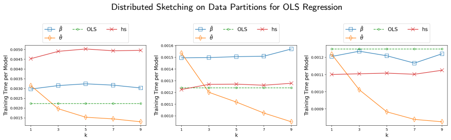
Summary. The paper studies distributed sketching for OLS under fixed design, but with sketches formed on row-partitioned blocks rather than on the full matrix. It defines three estimators (full OLS, averaged whole-data sketches, and averaged block sketches) and introduces the scalar D measuring average relative leverage / Burg-type divergence among the block Gram matrices. Theorem 3.3 gives an exact excess-loss formula B_ heta = (σ^{2}/k)(n-kd)/(m-d-1)·D + σ^{2}(D-d) for the averaged block-sketch estimator; the formula recovers the known whole-data result of Bartan & Pilanci when k=1 and is smaller whenever D is close to d. A high-probability out-of-sample bound (Remark 3.5) and an expectation of D under Gaussian design (Remark 3.4) are also supplied. Numerical experiments on three scikit-learn data sets illustrate a U-shaped gap versus k and the expected runtime reduction.

Significance. If the exact characterization holds under the stated assumptions, the work supplies a clean, non-asymptotic comparison between whole-data and partitioned sketching that was previously missing. The derivation is fully explicit (roadmap in §4, Claims 4.1–4.7, Wishart inverse moments, Vershynin singular-value bounds) and the quantity D has transparent interpretations via Burg divergence and relative leverage scores. The runtime advantage of block sketching is both theoretically clear (O(mdn/k) versus O(mdn)) and empirically confirmed. These are genuine, usable contributions for the distributed-sketching literature, provided the invertibility hypothesis is respected or relaxed.

major comments (2)

Standing assumption in §2 (and used throughout Claims 4.1, 4.5–4.6 and the definition of D) requires that every block Gram matrix X_i^ op X_i is invertible with probability one. Appendix C explicitly records that this fails on sparse real data (e.g., Digit under down-sampling). When a block is rank-deficient the local OLS solutions, residual orthogonality, Wishart expectations and the scalar D itself become undefined, so the exact identity of Theorem 3.3 and the comparison B_ heta ≤ B_eta hold only for partitions that keep all blocks full rank. The limitation is load-bearing for the central claim; either a regularized analysis or a clear statement of the domain of validity is needed before the result can be regarded as generally applicable.
Theorem 3.3 and the subsequent comparison with B_eta are stated for fixed design. Remark 3.4 supplies E[D] only under i.i.d. Gaussian rows; no analogous control is given for the heterogeneous or sparse regimes that the introduction itself flags as the setting where D may be large. Without such a bound (or an experiment that deliberately constructs large-D partitions) it remains unclear how often the claimed regime B_ heta ≤ B_eta actually occurs outside the i.i.d. case.

minor comments (5)

Abstract and first paragraph of §1 omit the standing invertibility hypothesis; a one-sentence caveat would prevent over-reading of the exact formula.
Notation for the three estimators (α̂*, β̄, θ̄) is introduced late; a short table or display early in §2 would help.
Figure 1 caption should state that excess loss is estimated on the given training matrix (in-sample), not out-of-sample, to avoid confusion with Remark 3.5.
Typographical inconsistencies appear throughout (missing spaces after commas, “Thispaper”, “OLSestimators”, etc.); a careful copy-edit is needed.
Appendix C mentions SRHT only for the whole-data estimator; a brief note on whether SRHT can be applied inside each block would round out the runtime discussion.

Circularity Check

0 steps flagged · score 0.0 of 10

No circularity: exact excess-loss formula of Theorem 3.3 is obtained by direct (non-fitted) expectation calculations under stated Gaussian/fixed-design assumptions, adapting an external lemma without self-reference.

full rationale

The central claim (Theorem 3.3) equates the excess risk of the averaged partitioned-sketch estimator to the closed-form expression B_θ involving the data-dependent scalar D. The derivation (Section 4 roadmap + Claims 4.1–4.7 + Appendices A–B) proceeds by expanding the squared loss, using residual orthogonality, independence of Gaussian sketches from residuals, and known Wishart inverse expectations; every algebraic step is exhibited and does not presuppose the target formula. D itself is defined from the block Gram matrices (Eq. 6) and is not tuned to force the claim. The only external ingredient is the adaptation of Bartan & Pilanci (2023) Lemma 1 to each block (Claim 4.5), which is an independent, non-overlapping citation whose hypotheses are restated and verified. No parameter is fitted to data and then re-presented as a prediction; no uniqueness theorem or ansatz is imported from the present authors; the comparison B_θ ≦ B_β is a direct algebraic consequence of the two closed forms when D is near d. The standing invertibility assumption is a domain restriction, not a circular definition. Consequently the derivation chain is self-contained and non-circular.

Assumptions & free parameters 1 free parameters · 5 assumptions · 1 invented entities

The result rests on standard fixed-design OLS assumptions, Gaussian sketching, and the technical requirement that every block Gram is invertible. No numerical constants are fitted to data to obtain B_θ; m and k are free design choices. D is a derived diagnostic, not a free parameter. The only non-standard modeling choice is the even row partition of a fixed design matrix.

free parameters (1)

sketch size m and partition count k
User-chosen design parameters that appear in B_θ; not fitted to observations but control the accuracy–cost trade-off.

assumptions (5)

domain assumption Fixed design: X is non-random; labels Y = Xα* + E with i.i.d. noise of variance σ².
Stated in §2; all excess-loss identities are conditional on this model.
domain assumption Sketch matrices have i.i.d. N(0,1/m) entries; m > d+1 (and p ≥ m).
Required for Wishart inverse moments used in Claims 4.5–4.6 and Theorem 3.3.
domain assumption With probability one every X_iᵀX_i is invertible (full column rank).
Standing assumption §2; without it D and the local OLS maps are undefined. Authors note failures on sparse data (Appendix C).
ad hoc to paper Even row partition with pk = n (extra rows discarded).
Convenience assumption used throughout the exact formula; uneven partitions are not analyzed.
standard math Classical Wishart inverse expectation and Vershynin singular-value bounds.
Invoked via Petersen et al. and Vershynin (2012) for Claims 4.5(c) and Remark 3.5.

invented entities (1)

Divergence D = (1/k²) Σ_{i,j} tr[(X_iᵀX_i)(X_jᵀX_j)^{-1}]
purpose: Scalar that quantifies heterogeneity of block Gram matrices and appears as the leading factor in B_θ.
Defined in Eq. (6); linked to Burg divergence and relative leverage scores but introduced specifically for this analysis. Independent evidence is limited to the algebraic lower bound D ≥ d (Lemma 2.1).

how reviews work

0 comments

Cite this review

Pith. "Pith review of Distributed Sketching on Data Partitions for OLS Regression." pith.science (2026). https://pith.science/paper/T7DDPEEI

@misc{pith2026260707888,
  author       = {Pith},
  title        = {Pith review of: Distributed Sketching on Data Partitions for OLS Regression},
  year         = {2026},
  howpublished = {\url{https://pith.science/paper/T7DDPEEI}},
  note         = {Machine review of arXiv:2607.07888}
}

read the original abstract

This paper studies distributed sketching for ordinary least squares (OLS) regression, an approach that distributes small sketches of a large data set over multiple machines to separately construct OLS estimators and average them. Unlike prior studies that consider sketching on the whole data set, we consider sketching on partitioned subsets to further reduce computational cost. Under the fixed design setting, we characterize the exact excess loss of the averaged OLS estimator. Results show that this loss is comparable to the established loss for sketching on the whole data set when the divergence among subset covariances is small.

Figures

Figures reproduced from arXiv: 2607.07888 by the authors.

**Figure 2.** Training Time per estimator versus 𝑘 on Digit (left), House (mid) and Cover (right) to build 𝜃̄, each data set was evenly partitioned based on the default data order, and the few extra 𝑛 − 𝑝𝑘 points were abandoned. The loss versus 𝑘 is shown in [PITH_FULL_IMAGE:figures/full_fig_p006_2.png] view at source ↗

**Figure 3.** Training Time per estimator versus 𝑘 on Digit, with 𝑛 = 1024 (left), 𝑛 = 256 (mid) and 𝑛 = 128 (right). Appendix C: Additional Numerical Results We report two additional observations here. First, a popular way to speed up Gaussian sketching is to apply faster sketching methods like Subsampled Randomized Hadamard Transform (SRHT). However, SRHT is not always faster, for its time complexity is 𝑂(𝑛𝑑 log 𝑛) which is mor… view at source ↗

Discussion (0). Sign in to comment.

Reference graph

Works this paper leans on

8 extracted references · 8 canonical work pages

[1]

, author=

Introduction to the non-asymptotic analysis of random matrices. , author=

work page
[2]

Low-rank kernel learning with bregman matrix divergences , author=. J. Machine Learning Research , volume=

work page
[3]

Advances in Neural Information Processing Systems , volume=

Fast exact leverage score sampling from Khatri-Rao products with applications to tensor decomposition , author=. Advances in Neural Information Processing Systems , volume=

work page
[4]

The Annals of Statistics , pages=

Estimation of a covariance matrix under Stein's loss , author=. The Annals of Statistics , pages=. 1985 , publisher=

work page 1985
[5]

IEEE Transactions on Information Theory , volume=

Distributed sketching for randomized optimization: Exact characterization, concentration, and lower bounds , author=. IEEE Transactions on Information Theory , volume=. 2023 , publisher=

work page 2023
[6]

Advances in Neural Information Processing Systems , volume=

Distributed least squares in small space via sketching and bias reduction , author=. Advances in Neural Information Processing Systems , volume=

work page
[7]

GPU-Parallelizable Randomized Sketch-and-Precondition for Linear Regression using Sparse Sign Sketches

GPU-Parallelizable Randomized Sketch-and-Precondition for Linear Regression using Sparse Sign Sketches , author=. arXiv preprint arXiv:2506.03070 , year=

work page Pith review arXiv
[8]

Technical University of Denmark , volume=

The matrix cookbook , author=. Technical University of Denmark , volume=

work page

Pith tools

Reviewed July 10, 2026 · model on record in the stance chip above.

[1] [1]

, author=

Introduction to the non-asymptotic analysis of random matrices. , author=

work page

[2] [2]

Low-rank kernel learning with bregman matrix divergences , author=. J. Machine Learning Research , volume=

work page

[3] [3]

Advances in Neural Information Processing Systems , volume=

Fast exact leverage score sampling from Khatri-Rao products with applications to tensor decomposition , author=. Advances in Neural Information Processing Systems , volume=

work page

[4] [4]

The Annals of Statistics , pages=

Estimation of a covariance matrix under Stein's loss , author=. The Annals of Statistics , pages=. 1985 , publisher=

work page 1985

[5] [5]

IEEE Transactions on Information Theory , volume=

Distributed sketching for randomized optimization: Exact characterization, concentration, and lower bounds , author=. IEEE Transactions on Information Theory , volume=. 2023 , publisher=

work page 2023

[6] [6]

Advances in Neural Information Processing Systems , volume=

Distributed least squares in small space via sketching and bias reduction , author=. Advances in Neural Information Processing Systems , volume=

work page

[7] [7]

GPU-Parallelizable Randomized Sketch-and-Precondition for Linear Regression using Sparse Sign Sketches

GPU-Parallelizable Randomized Sketch-and-Precondition for Linear Regression using Sparse Sign Sketches , author=. arXiv preprint arXiv:2506.03070 , year=

work page Pith review arXiv

[8] [8]

Technical University of Denmark , volume=

The matrix cookbook , author=. Technical University of Denmark , volume=

work page