REVIEW 2 major objections 5 minor 80 references
A single global radial-basis field, shaped by local attractor geometry, recovers the long-term statistics of chaotic flows without using the governing equations.
Reviewed by Pith at T0; open to challenge. T0 means a machine referee read the full paper against a public rubric. the ladder, T0–T4 →
T0 review · grok-4.5
2026-07-10 05:07 UTC pith:HPNGWJ4R
load-bearing objection Solid non-intrusive ROM that matches intrusive local Galerkin and neural baselines on invariant measures; the corrector is a real but honestly quantified limitation, not a fatal one. the 2 major comments →
Manifold-adapted radial basis functions for reduced-order modelling of chaotic flows
The pith
A machine-rendered reading of the paper's core claim, the machinery that carries it, and where it could break.
Core claim
A non-intrusive reduced-order model that shapes a radial-basis library by clustering the attractor and fitting the reduced velocity by one global regularised least-squares solve yields an explicit, differentiable vector field that reproduces the invariant measure of chaotic and quasiperiodic flows as faithfully as an intrusive quantised-local Galerkin model of the same dimension, without ever projecting the governing equations.
What carries the argument
Manifold-adapted anisotropic radial basis library: kernels inherit each cluster’s local principal directions and widths so they elongate along the attractor and stay thin normal to it; the reduced velocity is then recovered by a single global ridge-regularised regression onto this library, producing one continuous differentiable field rather than switched local models.
Load-bearing premise
That the kinematic corrector, needed because the pure radial-basis field under-recovers transverse contraction and decays away from the data, stays inactive on the attractor and does not bias the reported long-term statistics.
What would settle it
On a system whose excursions routinely leave the training support, integrate the bare learned field without the corrector for thousands of Lyapunov times and check whether the energy density, spectrum, or leading Lyapunov exponents systematically deviate from the full-order reference while the reported corrector magnitude remains large.
Editorial analysis
A structured set of objections, weighed in public.
Referee Report
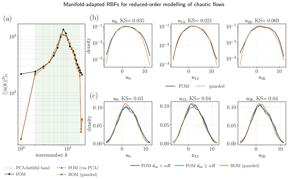
Summary. The paper proposes a non-intrusive reduced-order model for chaotic and quasiperiodic flows: reduced coordinates (global POD when needed) are clustered, local principal directions shape anisotropic Gaussian RBF kernels, and a single global regularised least-squares fit yields an explicit, differentiable reduced vector field. Integration is stabilised by a kinematic trust-region corrector whose relative magnitude is reported. On Lorenz-63 the model recovers the attractor, marginals, and the positive/neutral Lyapunov exponents (analytic Jacobian) while under-recovering transverse contraction; on Lorenz-96 short-term VPT is competitive with tuned RC/GRU/LSTM baselines and the invariant measure is reproduced; on chaotic Kuramoto–Sivashinsky and quasiperiodic Kolmogorov flow the energy density and spectrum match an intrusive quantised-local Galerkin model of the same dimension and improve on a global Galerkin projection, without projecting the governing equations.
Significance. If the results hold, the work supplies a practical middle path between opaque neural/reservoir forecasters and intrusive Galerkin ROMs: an explicit, differentiable, non-intrusive field that is competitive on short-term skill and matches equation-based local Galerkin models on long-term statistics. Strengths that raise the contribution above a pure methods note include (i) Lyapunov spectra read from the analytic Jacobian rather than trajectory estimates, (ii) systematic diagnosis of under-contraction via divergence and λ3, (iii) data-driven calibration of the corrector with on-attractor inactivity checks (KS, spectra, autocorrelation), (iv) head-to-head comparison against both published neural baselines and the ql-ROM/g-ROM of Colanera & Magri, and (v) open code and data. The manifold-adapted library (clustering shapes kernels, not switched local dynamics) is a clear design choice relative to cluster-based ROMs and sparse regression/operator inference.
major comments (2)
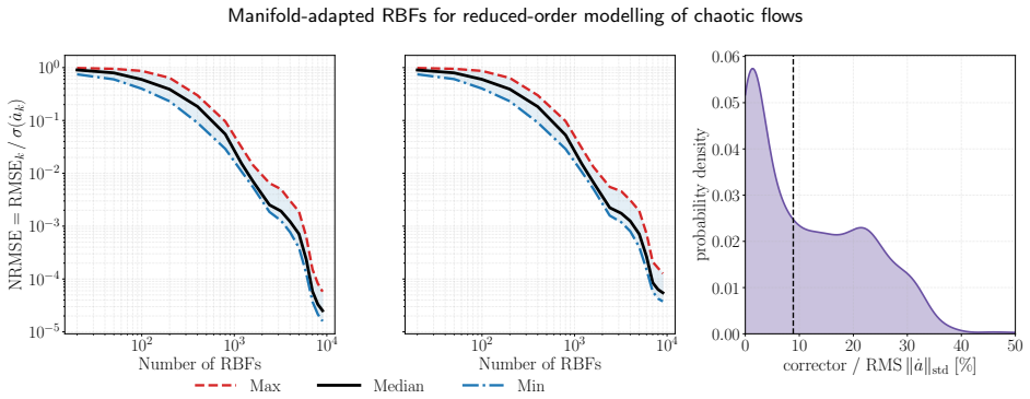
- [§3.1, Eq. (15), Appendix A] §3.1 (Fig. 7), §2.3.3 Eq. (15), and Appendix A: the pure RBF field systematically under-recovers transverse contraction (λ3 ≈ −12 vs −14.57; divergence sum ≈ −11 vs −13.67 on Lorenz-63), and kernels decay off the data so the learned Jacobian lacks restoring eigenvalues. Long-time invariant-measure results that underwrite the central claim (Figs. 10–12; KS distances, spectra, energy densities) are obtained from the composite field f+c. The paper is transparent and verifies on-attractor inactivity within tolerance, but the main text should state, for each system, whether pure f remains bounded under the reported integration length and should report the median corrector/RMS∥ȧ∥ ratio for the headline runs in the main results (currently largely confined to Appendix B density plots). Without that, readers cannot judge how far each statistic rests on the learned field versus the safeguard.
- [§2.2.3, Appendix B] §2.2.3 and Appendix B: selection of K is only partly automatic. BIC supplies a range; geometric/dynamical distinctness is then judged by eye (“rise clearly above baseline”). For Lorenz-96 the marginal BIC has no elbow and K=10 is fixed “by convention” (Fig. 16). Because the manifold-adapted claim rests on the clusters correctly reading local geometry, a short sensitivity study (invariant-measure diagnostics at neighbouring K, or at K=1 isotropic) for the headline systems would show that the reported statistics are not an artefact of a hand-chosen partition.
minor comments (5)
- [Abstract, §1] Abstract and §1: the phrase “reproduces the long-term statistics… without any use of the governing equations” is accurate for the fit, but a brief clause that long integrations use the reported kinematic corrector would align the abstract with the body and with the honesty of §2.3.3.
- [§3.2, Fig. 9] Fig. 9 caption and text: the violin comparison is carefully caveated (baselines span hyperparameters; RBF spans initial conditions), but the main-text sentence “mid-field” could explicitly point the reader to the best-tuned baseline medians so the figure is not misread as a hyperparameter-averaged contest.
- [§2.3.1–2.3.2] §2.3.1–2.3.2: the normal-width floor and the ridge λ (leave-one-out then long-term confirmation) are important conditioning choices; a one-line default recipe (or the values used per system) in a small table would aid reproduction beyond the GitHub release.
- [Figs. 1, 3] Fig. 1 and Fig. 3 are helpful; ensure axis labels and the distinction between time sampling vs arc-length sampling remain legible at journal column width.
- [§3.3, Refs.] References: the ql-ROM comparison is central; ensure the published Colanera & Magri (2025) citation and any shared data protocols are stated so the energy-density rescaling on Kolmogorov (Fig. 12) is fully reproducible.
Circularity Check
No load-bearing circularity: the RBF field is a standard least-squares fit to trajectory data, evaluated on independent long-term statistics, known Lyapunov spectra, and external published benchmarks; the corrector is an explicit, reported safeguard rather than a hidden redefinition of the claim.
full rationale
The paper is a methodological contribution that constructs an explicit vector field by global regularised least-squares regression of reduced velocities onto a geometry-adapted RBF library (eqs. 11–14), then integrates the composite field and compares the resulting invariant measure (energy densities, spectra, marginals) and short-term skill (VPT) against independent references: the known Lorenz-63 Lyapunov spectrum, the published neural/reservoir numbers of Vlachas et al., and the intrusive ql-ROM/g-ROM of Colanera & Magri. None of these comparisons is forced by construction; the fit is to instantaneous velocities on the training snapshots, while the reported quantities are long-horizon occupation measures and analytic Jacobian eigenvalues that a merely interpolating field need not recover. The kinematic corrector (eq. 15, App. A) is calibrated from residual outward drift on the same training cloud and is therefore data-dependent, yet the paper treats it as an external patch, reports its relative magnitude on every case, and verifies that on-attractor statistics remain unbiased within KS tolerance. This is transparent engineering, not a self-definitional loop or a fitted constant renamed as prediction. There are no uniqueness theorems, no load-bearing self-citations of prior author results, and no renaming of a known empirical pattern. The single minor note is that the corrector strength is itself a statistic of the training residual; because the paper never claims the pure RBF field alone produces the reported long-term statistics on systems that leave the support, this does not elevate the score above 1.
Axiom & Free-Parameter Ledger
free parameters (6)
- number of clusters K
- tangent width multiplier α_t
- ridge penalty λ
- number of RBF centres n_c
- corrector parameters (k, p, α, q)
- POD energy threshold
axioms (4)
- domain assumption Reduced coordinates evolve under a closed Markovian velocity field f(a) that can be learned from the projected trajectory alone.
- domain assumption Local principal directions of K-means clusters furnish a faithful approximate tangent space of the attractor for shaping anisotropic kernels.
- standard math A radial-basis sum is a universal approximator on compact sets and remains sufficiently accurate when kernels are elongated along the data cloud.
- ad hoc to paper The kinematic corrector of eq. (15) can be made inactive on the attractor while restoring boundedness off it without biasing invariant measures.
invented entities (2)
-
manifold-adapted anisotropic RBF library
independent evidence
-
kinematic trust-region corrector
no independent evidence
read the original abstract
Chaotic systems often evolve on a low-dimensional attractor whose geometry varies from one region to another. We propose a non-intrusive reduced-order model that reads this local geometry by clustering and uses it to shape a radial basis library whose kernels adapt to each region. Fitting the reduced velocity onto this library by one global regularised least-squares solve gives an explicit, differentiable vector field that reproduces the long-term statistics, that is, the invariant measure, without any use of the governing equations. Since a radial basis field decays away from the data and cannot by itself return an escaped state, the integration is stabilised by a kinematic corrector whose magnitude is reported as a measure of how far each result rests on the learned field rather than on the corrector. On Lorenz-63 the model recovers the attractor, its marginal densities, and the positive and neutral Lyapunov exponents, while under-recovering the strong transverse contraction. On Lorenz-96 its valid prediction time is competitive with tuned neural-network and reservoir-computing forecasters, and the invariant measure is reproduced on both the full state and a reduced observable. On the Kuramoto--Sivashinsky equation and the quasiperiodic Kolmogorov flow the model matches the energy distribution and spectrum of an intrusive quantised-local Galerkin model, and improves on a global Galerkin projection of the same dimension, without ever projecting the governing equations.
Figures




Reference graph
Works this paper leans on
-
[1]
G. K. Vallis, Atmospheric and Oceanic Fluid Dynamics: Fundamentals and Large-Scale Circulation, 2nd ed., Cambridge University Press, 2017
work page 2017
-
[2]
Kalnay, Atmospheric Modeling, Data Assimilation and Predictability, Cambridge University Press, 2003
E. Kalnay, Atmospheric Modeling, Data Assimilation and Predictability, Cambridge University Press, 2003
work page 2003
-
[3]
P. Bauer, A. Thorpe, G. Brunet, The quiet revolution of numerical weather prediction, Nature 525 (2015) 47–55. doi:10.1038/nature14956
-
[4]
S. B. Pope, Turbulent Flows, Cambridge University Press, 2000. doi:10.1017/CBO9780511840531
-
[5]
Frisch, Turbulence: The Legacy of A
U. Frisch, Turbulence: The Legacy of A. N. Kolmogorov, Cambridge University Press, 1995
work page 1995
-
[6]
E. N. Lorenz, Deterministic nonperiodic flow, Journal of the Atmospheric Sciences 20 (1963) 130–141. doi:10.1175/1520-0469(1963) 020<0130:DNF>2.0.CO;2
-
[7]
S. H. Strogatz, Nonlinear Dynamics and Chaos: With Applications to Physics, Biology, Chemistry, and Engineering, 2nd ed., Westview Press, 2015
work page 2015
-
[8]
P. Moin, K. Mahesh, Direct numerical simulation: a tool in turbulence research, Annual Review of Fluid Mechanics 30 (1998) 539–578. doi:10.1146/annurev.fluid.30.1.539
-
[9]
T. Ishihara, T. Gotoh, Y. Kaneda, Study of high–reynolds number isotropic turbulence by direct numerical simulation, Annual Review of Fluid Mechanics 41 (2009) 165–180
work page 2009
-
[10]
H. Choi, P. Moin, Grid-point requirements for large eddy simulation: Chapman’s estimates revisited, Physics of Fluids 24 (2012) 011702
work page 2012
-
[11]
P. R. Spalart, Strategies for turbulence modelling and simulations, International Journal of Heat and Fluid Flow 21 (2000) 252–263
work page 2000
-
[12]
S. L. Brunton, B. R. Noack, Closed-loop turbulence control: Progress and challenges, Applied Mechanics Reviews 67 (2015) 050801. doi:10.1115/1.4031175
-
[13]
Evensen, Data Assimilation: The Ensemble Kalman Filter, 2nd ed., Springer, 2009
G. Evensen, Data Assimilation: The Ensemble Kalman Filter, 2nd ed., Springer, 2009
work page 2009
-
[14]
P. Benner, S. Gugercin, K. Willcox, A survey of projection-based model reduction methods for parametric dynamical systems, SIAM Review 57 (2015) 483–531. doi:10.1137/130932715
-
[15]
C. W. Rowley, S. T. M. Dawson, Model reduction for flow analysis and control, Annual Review of Fluid Mechanics 49 (2017) 387–417. doi:10.1146/annurev-fluid-010816-060042
-
[16]
G. Benettin, L. Galgani, A. Giorgilli, J.-M. Strelcyn, Lyapunov characteristic exponents for smooth dynamical systems and for hamiltonian systems; a method for computing all of them. part 1: Theory, Meccanica 15 (1980) 9–20. doi:10.1007/BF02128236
-
[17]
E. N. Lorenz, The predictability of a flow which possesses many scales of motion, Tellus 21 (1969) 289–307. doi:10.3402/tellusa.v21i3. 10086
-
[18]
P. R. Vlachas, W. Byeon, Z. Y. Wan, T. P. Sapsis, P. Koumoutsakos, Data-driven forecasting of high-dimensional chaotic systems with long short-term memory networks, Proceedings of the Royal Society A 474 (2018) 20170844. doi:10.1098/rspa.2017.0844
-
[19]
J.-P. Eckmann, D. Ruelle, Ergodic theory of chaos and strange attractors, Reviews of Modern Physics 57 (1985) 617–656. doi:10.1103/ RevModPhys.57.617
work page 1985
-
[20]
M. Schlegel, B. R. Noack, On long-term boundedness of galerkin models, Journal of Fluid Mechanics 765 (2015) 325–352. doi:10.1017/jfm. 2014.736
work page doi:10.1017/jfm 2015
-
[21]
J. Pathak, Z. Lu, B. R. Hunt, M. Girvan, E. Ott, Using machine learning to replicate chaotic attractors and calculate lyapunov exponents from data, Chaos: An Interdisciplinary Journal of Nonlinear Science 27 (2017) 121102. doi:10.1063/1.5010300. M. Pérez Cuadrado et al.:Preprint submitted to ElsevierPage 29 of 31 Manifold-adapted RBFs for reduced-order mo...
-
[22]
P. R. Vlachas, J. Pathak, B. R. Hunt, T. P. Sapsis, M. Girvan, E. Ott, P. Koumoutsakos, Backpropagation algorithms and reservoir computing in recurrent neural networks for the forecasting of complex spatiotemporal dynamics, Neural Networks 126 (2020) 191–217. doi:10.1016/j.neunet.2020.02.016
-
[23]
J. Pathak, B. Hunt, M. Girvan, Z. Lu, E. Ott, Model-free prediction of large spatiotemporally chaotic systems from data: A reservoir computing approach, Physical Review Letters 120 (2018) 024102. doi:10.1103/PhysRevLett.120.024102
-
[24]
Sirovich, Turbulence and the dynamics of coherent structures
L. Sirovich, Turbulence and the dynamics of coherent structures. I. Coherent structures, Quarterly of Applied Mathematics 45 (1987) 561–571. doi:10.1090/qam/910462
- [25]
-
[26]
A. Colanera, L. Magri, Quantized local reduced-order modeling in time (ql-rom), Computer Methods in Applied Mechanics and Engineering 447 (2025) 118393. doi:10.1016/j.cma.2025.118393
-
[27]
D. Amsallem, M. J. Zahr, C. Farhat, Nonlinear model order reduction based on local reduced-order bases, International Journal for Numerical Methods in Engineering 92 (2012) 891–916. doi:10.1002/nme.4371
-
[28]
K. Lee, K. T. Carlberg, Model reduction of dynamical systems on nonlinear manifolds using deep convolutional autoencoders, Journal of Computational Physics 404 (2020) 108973. doi:10.1016/j.jcp.2019.108973
-
[29]
S. L. Brunton, J. L. Proctor, J. N. Kutz, Discovering governing equations from data by sparse identification of nonlinear dynamical systems, Proceedings of the National Academy of Sciences 113 (2016) 3932–3937. doi:10.1073/pnas.1517384113
-
[30]
J.-C. Loiseau, S. L. Brunton, Constrained sparse galerkin regression, Journal of Fluid Mechanics 838 (2018) 42–67. doi:10.1017/jfm.2017. 823
-
[31]
B. Peherstorfer, K. Willcox, Data-driven operator inference for nonintrusive projection-based model reduction, Computer Methods in Applied Mechanics and Engineering 306 (2016) 196–215. doi:10.1016/j.cma.2016.03.025
-
[32]
D. S. Broomhead, D. Lowe, Multivariable functional interpolation and adaptive networks, Complex Systems 2 (1988) 321–355
work page 1988
-
[33]
M.Casdagli, Nonlinearpredictionofchaotictimeseries, PhysicaD:NonlinearPhenomena35(1989)335–356.doi: 10.1016/0167-2789(89) 90074-2
-
[34]
E. Kaiser, B. R. Noack, L. Cordier, A. Spohn, M. Segond, M. Abel, G. Daviller, J. Östh, S. Krajnović, R. K. Niven, Cluster-based reduced-order modelling of a mixing layer, Journal of Fluid Mechanics 754 (2014) 365–414. doi:10.1017/jfm.2014.355
-
[35]
D. Fernex, B. R. Noack, R. Semaan, Cluster-based network modeling: From snapshots to complex dynamical systems, Science Advances 7 (2021) eabf5006. doi:10.1126/sciadv.abf5006
-
[36]
C.Eckart,G.Young, Theapproximationofonematrixbyanotheroflowerrank, Psychometrika1(1936)211–218.doi: 10.1007/BF02288367
-
[37]
F. Ginelli, P. Poggi, A. Turchi, H. Chaté, R. Livi, A. Politi, Characterizing dynamics with covariant Lyapunov vectors, Physical Review Letters 99 (2007) 130601. doi:10.1103/PhysRevLett.99.130601
-
[38]
Q. L. Li-Hu, G. Y. Cornejo Maceda, A. Ianiro, S. Discetti, Divide and conquer: Cluster and manifold-based interpretation of complex flows, arXiv preprint arXiv:2601.05117 (2026).arXiv:2601.05117
work page internal anchor Pith review arXiv 2026
-
[39]
S. P. Lloyd, Least squares quantization in PCM, IEEE Transactions on Information Theory 28 (1982) 129–137. doi:10.1109/TIT.1982. 1056489
- [40]
-
[41]
J. L. Lumley, The structure of inhomogeneous turbulent flows, in: A. M. Yaglom, V. I. Tatarski (Eds.), Atmospheric Turbulence and Radio Wave Propagation, Nauka, Moscow, 1967, pp. 166–178
work page 1967
-
[42]
G. Berkooz, P. Holmes, J. L. Lumley, The proper orthogonal decomposition in the analysis of turbulent flows, Annual Review of Fluid Mechanics 25 (1993) 539–575. doi:10.1146/annurev.fl.25.010193.002543
-
[43]
J. Burkardt, M. Gunzburger, H.-C. Lee, POD and CVT-based reduced-order modeling of Navier–Stokes flows, Computer Methods in Applied Mechanics and Engineering 196 (2006) 337–355. doi:10.1016/j.cma.2006.04.004
-
[44]
P. L. Zador, Asymptotic quantization error of continuous signals and the quantization dimension, IEEE Transactions on Information Theory 28 (1982) 139–149. doi:10.1109/TIT.1982.1056490
-
[45]
A. Gersho, Asymptotically optimal block quantization, IEEE Transactions on Information Theory 25 (1979) 373–380. doi:10.1109/TIT. 1979.1056067
work page doi:10.1109/tit 1979
-
[46]
S. Graf, H. Luschgy, Foundations of Quantization for Probability Distributions, volume 1730 ofLecture Notes in Mathematics, Springer, 2000. doi:10.1007/BFb0103945
-
[47]
L.-S. Young, What are SRB measures, and which dynamical systems have them?, Journal of Statistical Physics 108 (2002) 733–754. doi:10.1023/A:1019762724717
-
[48]
Schwarz,Estimating the dimension of a model, The annals of statistics, 6 (1978), pp
G. Schwarz, Estimating the dimension of a model, The Annals of Statistics 6 (1978) 461–464. doi:10.1214/aos/1176344136
- [49]
-
[50]
V. Satopaa, J. Albrecht, D. Irwin, B. Raghavan, Finding a “kneedle” in a haystack: Detecting knee points in system behavior, in: 2011 31st International Conference on Distributed Computing Systems Workshops (ICDCSW), IEEE, 2011, pp. 166–171. doi:10.1109/ICDCSW.2011. 20
-
[51]
N. Kambhatla, T. K. Leen, Dimension reduction by local principal component analysis, Neural Computation 9 (1997) 1493–1516. doi:10.1162/neco.1997.9.7.1493
-
[52]
Å. Björck, G. H. Golub, Numerical methods for computing angles between linear subspaces, Mathematics of Computation 27 (1973) 579–594. doi:10.1090/S0025-5718-1973-0348991-3
-
[53]
R. J. Bell, P. Dean, Atomic vibrations in vitreous silica, Discussions of the Faraday Society 50 (1970) 55–61. doi:10.1039/DF9705000055. M. Pérez Cuadrado et al.:Preprint submitted to ElsevierPage 30 of 31 Manifold-adapted RBFs for reduced-order modelling of chaotic flows
-
[54]
C. A. Micchelli, Interpolation of scattered data: Distance matrices and conditionally positive definite functions, Constructive Approximation 2 (1986) 11–22. doi:10.1007/BF01893414
-
[55]
M.J.D.Powell, Radialbasisfunctionsformultivariableinterpolation:areview, in:J.C.Mason,M.G.Cox(Eds.),AlgorithmsforApproximation, Clarendon Press, Oxford, 1987, pp. 143–167
work page 1987
-
[56]
J. Park, I. W. Sandberg, Universal approximation using radial-basis-function networks, Neural Computation 3 (1991) 246–257. doi:10.1162/neco.1991.3.2.246
-
[57]
E. J. Hartman, J. D. Keeler, J. M. Kowalski, Layered neural networks with Gaussian hidden units as universal approximations, Neural Computation 2 (1990) 210–215. doi:10.1162/neco.1990.2.2.210
-
[58]
P. C. Mahalanobis, On the generalised distance in statistics, Proceedings of the National Institute of Sciences of India 2 (1936) 49–55
work page 1936
-
[59]
M. P. Wand, M. C. Jones, Kernel Smoothing, number 60 in Monographs on Statistics and Applied Probability, Chapman & Hall/CRC, London, 1995
work page 1995
-
[60]
T. Berry, J. Harlim, Variable bandwidth diffusion kernels, Applied and Computational Harmonic Analysis 40 (2016) 68–96. doi:10.1016/j. acha.2015.01.001
work page doi:10.1016/j 2016
-
[61]
T. F. Gonzalez, Clustering to minimize the maximum intercluster distance, Theoretical Computer Science 38 (1985) 293–306. doi:10.1016/ 0304-3975(85)90224-5
work page 1985
-
[62]
R. Schaback, Error estimates and condition numbers for radial basis function interpolation, Advances in Computational Mathematics 3 (1995) 251–264. doi:10.1007/BF02432002
-
[63]
G. E. Fasshauer, Meshfree Approximation Methods with MATLAB, volume 6 ofInterdisciplinary Mathematical Sciences, World Scientific, Singapore, 2007
work page 2007
-
[64]
T. Poggio, F. Girosi, Networks for approximation and learning, Proceedings of the IEEE 78 (1990) 1481–1497. doi:10.1109/5.58326
-
[65]
M. J. L. Orr, Regularization in the selection of radial basis function centers, Neural Computation 7 (1995) 606–623. doi:10.1162/neco. 1995.7.3.606
-
[66]
A. E. Hoerl, R. W. Kennard, Ridge regression: biased estimation for nonorthogonal problems, Technometrics 12 (1970) 55–67. doi:10.1080/00401706.1970.10488634
- [67]
-
[68]
doi:10.1007/978-0-387-84858-7
-
[69]
P. C. Hansen, Rank-Deficient and Discrete Ill-Posed Problems: Numerical Aspects of Linear Inversion, SIAM Monographs on Mathematical Modeling and Computation, Society for Industrial and Applied Mathematics, Philadelphia, 1998. doi:10.1137/1.9780898719697
-
[70]
doi:10.1080/00401706.1974.10489157
D.M.Allen, Therelationshipbetweenvariableselectionanddataaugmentationandamethodforprediction, Technometrics16(1974)125–127. doi:10.1080/00401706.1974.10489157
-
[71]
G. H. Golub, M. Heath, G. Wahba, Generalized cross-validation as a method for choosing a good ridge parameter, Technometrics 21 (1979) 215–223. doi:10.1080/00401706.1979.10489751
-
[72]
A. A. Kaptanoglu, J. L. Callaham, A. Aravkin, C. J. Hansen, S. L. Brunton, Promoting global stability in data-driven models of quadratic nonlinear dynamics, Physical Review Fluids 6 (2021) 094401. doi:10.1103/PhysRevFluids.6.094401
-
[73]
E. N. Lorenz, Predictability: a problem partly solved, in: Proceedings of the Seminar on Predictability, volume 1, ECMWF, Reading, UK, 1996, pp. 1–18
work page 1996
-
[74]
doi:10.1175/1520-0469(1998)055<0399:OSFSWO>2.0.CO;2
E.N.Lorenz,K.A.Emanuel, Optimalsitesforsupplementaryweatherobservations:Simulationwithasmallmodel, JournaloftheAtmospheric Sciences 55 (1998) 399–414. doi:10.1175/1520-0469(1998)055<0399:OSFSWO>2.0.CO;2
-
[75]
Y. Kuramoto, T. Tsuzuki, Persistent propagation of concentration waves in dissipative media far from thermal equilibrium, Progress of Theoretical Physics 55 (1976) 356–369. doi:10.1143/PTP.55.356
-
[76]
G. I. Sivashinsky, Nonlinear analysis of hydrodynamic instability in laminar flames—I. Derivation of basic equations, Acta Astronautica 4 (1977) 1177–1206. doi:10.1016/0094-5765(77)90096-0
-
[77]
R. Ghrist, Barcodes: the persistent topology of data, Bulletin of the American Mathematical Society 45 (2008) 61–75. doi:10.1090/ S0273-0979-07-01191-3
work page 2008
-
[78]
G.Carlsson, Topologyanddata, BulletinoftheAmericanMathematicalSociety46(2009)255–308.doi: 10.1090/S0273-0979-09-01249-X
-
[79]
Schreiber, Measuring information transfer, Physical Review Letters 85 (2000) 461–464
T. Schreiber, Measuring information transfer, Physical Review Letters 85 (2000) 461–464. doi:10.1103/PhysRevLett.85.461
-
[80]
H. K. Khalil, Nonlinear Systems, 3 ed., Prentice Hall, Upper Saddle River, NJ, 2002. M. Pérez Cuadrado et al.:Preprint submitted to ElsevierPage 31 of 31
work page 2002
discussion (0)
Sign in with ORCID, Apple, or X to comment. Anyone can read and Pith papers without signing in.