REVIEW 3 major objections 5 minor 27 references
Without prior knowledge of structural change, average rolling- and expanding-window demographic forecasts for a robust default.
Reviewed by Pith at T0; open to challenge. T0 means a machine referee read the full paper against a public rubric. the ladder, T0–T4 →
T0 review · grok-4.5
2026-07-14 11:02 UTC pith:UWF7DWOU
load-bearing objection Solid multi-country empirical guidance on a routine choice; the equal-weight hedge is practical but never formally tested against the better single scheme. the 3 major comments →
Age-specific demographic modeling and forecasting: Rolling window, expanding window, or both?
The pith
A machine-rendered reading of the paper's core claim, the machinery that carries it, and where it could break.
Core claim
In multi-country comparisons of age-specific mortality and fertility forecasts, the superior performance of either the rolling or the expanding window often persists across horizons, yet neither scheme dominates uniformly by sex, component, or country. An equal-weight combination of the two forecasts therefore provides a robust, tuning-free alternative that is never systematically inferior and frequently tracks or exceeds the better single scheme while reducing end-of-horizon volatility.
What carries the argument
Equal-weight ensemble (Eq. 3): the simple average of the rolling-window and expanding-window forecasts produced by the same functional time-series model, with no extra tuning parameter.
Load-bearing premise
A fixed half-and-half average is assumed to be a good enough hedge even though which window wins can change with horizon, sex, and the underlying model, and the paper does not test whether the average is statistically better than the better single scheme.
What would settle it
Re-run the same multi-country holdout design with formal horizon-wise tests of equal predictive ability; if the equal-weight combination is significantly worse than the better single scheme on a large share of country-horizon cells, the robustness claim fails.
Editorial analysis
A structured set of objections, weighed in public.
Referee Report
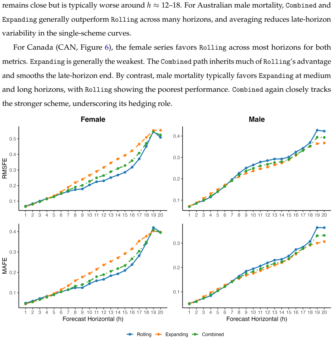
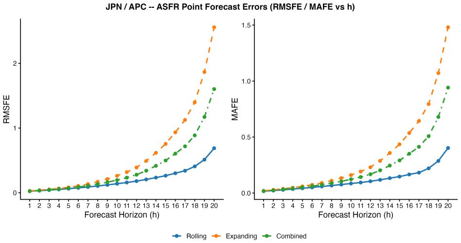
Summary. The paper compares rolling-window and expanding-window estimation schemes for age-specific mortality and fertility forecasting within a common functional time-series framework (Hyndman–Ullah, K=6), and proposes a fixed equal-weight average of the two forecasts (Eq. 3). Using multi-country data from the Human Mortality Database (23 countries) and Human Fertility Database (16 countries), with a fixed 20-year hold-out, it evaluates point accuracy (RMSFE, MAFE) and interval accuracy (ECP/CPD, interval score) over horizons h=1…20. Horizon-wise win-count heatmaps and country panels (Australia/Canada mortality; Canada/Japan fertility) show that no single scheme dominates uniformly: expanding (or combined) often leads for female mortality and for fertility, while rolling (or combined) often leads for male mortality and for mortality intervals. An appendix repeats the exercise under Lee–Carter and APC benchmarks. The central recommendation is that, absent prior information on structural stability, the equal-weight combination is a robust, tuning-free default.
Significance. The question of rolling versus expanding windows is practically important and under-studied in demographic forecasting; a transparent multi-country design with both point and interval metrics, sex-specific mortality, and an LC/APC sensitivity appendix is a genuine contribution. The equal-weight combination is simple, reproducible, and operationally attractive as a hedge when leadership changes with horizon, sex, or component. Code availability further strengthens the work. The main limitation is that the robustness claim rests on descriptive win counts and visual tracking rather than formal tests of equal predictive ability, so the statistical status of the combination as a default remains incompletely established.
major comments (3)
- Abstract and §6 claim that the equal-weight combination (Eq. 3) is a robust default that is “never systematically inferior” and frequently matches or exceeds the better single scheme. The supporting evidence is horizon-wise win-count heatmaps (Figs. 4, 7, 10, 13) and country line plots. These do not test equal predictive ability (e.g., Diebold–Mariano, MCS, or SPA). The paper itself notes that leadership changes with horizon, sex, and model class, yet never tests whether Combined is statistically better than, or not worse than, the better of Rolling/Expanding. Formal horizon-wise tests (or at least paired error differences with uncertainty) are needed to underwrite the central claim.
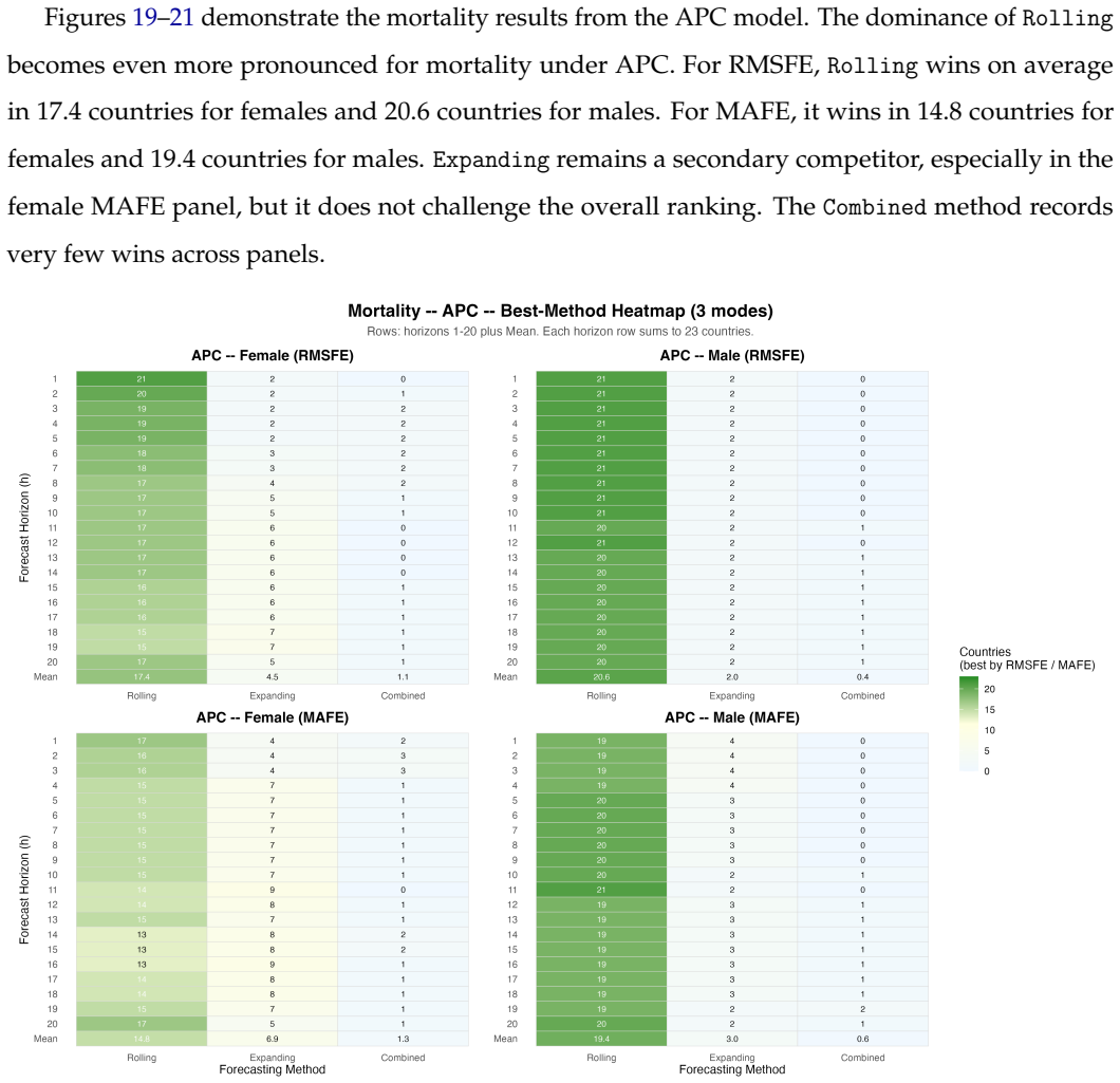
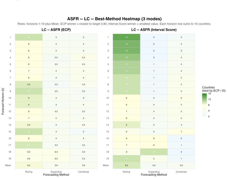
- The LC/APC appendix (Figs. 16–27 and interval tables) shows Combined rarely wins and often sits between the two single schemes, while Rolling dominates under LC and APC for mortality and LC-ASFR. The abstract/§6 recommendation that Combined is a robust default is therefore model-class dependent. The main text should qualify the claim by model class and state when the combination is recommended versus when a single scheme is preferred under lower-dimensional benchmarks.
- Eq. (3) fixes the combination weight at 1/2 with no data-driven alternative or sensitivity. Given that leadership changes with h, sex, and component, a short check of alternative fixed weights (e.g., 0.3/0.7) or a simple validation-based weight would show whether equal weight is special or merely convenient. Without this, the “tuning-free” virtue is clear but the optimality of 1/2 is unexamined.
minor comments (5)
- §5.1: interval evaluation uses h=1…19 because of the SD validation requirement, while point evaluation uses h=1…20; state this consistently in figure captions and text to avoid confusion.
- Country selection (continuous series through 1950) is reasonable but should be justified more explicitly as a design choice that may favor longer-history methods; a brief note on excluded countries would help.
- Notation: Yt(ui) is used for both raw and log rates in places; clarify the scale on which MAFE/RMSFE and interval scores are computed (original vs log).
- Figures 11–12 and 14–15 are dense; ensuring consistent axis scales and a single legend placement would improve readability.
- A few typos and awkward phrases remain (e.g., “panel countries,” “mean change”); a light copy-edit pass would help.
Circularity Check
No circularity: purely empirical multi-country comparison of rolling, expanding, and equal-weight combined forecasts on held-out data; no derivation that reduces to a fitted quantity by construction.
full rationale
The paper proposes a fixed equal-weight average of rolling- and expanding-window forecasts (Eq. 3) and evaluates it against the two single schemes using standard point (RMSFE, MAFE) and interval (ECP/CPD, interval score) metrics on multi-country holdout sets (last 20 years) for mortality and fertility, plus an LC/APC sensitivity appendix. All claims are comparative empirical statements about which scheme wins more often across horizons and countries; there is no first-principles derivation, uniqueness theorem, or fitted parameter that is then re-labeled as a prediction. Self-citations (Hyndman & Shang, Shang & Haberman, Shang & Xu) supply the functional time-series method, smoothing, and interval construction tools; they are not load-bearing for the target claim that the ½ combination is a robust default. The equal weight is an explicit, untuned ansatz, not a quantity fitted to the evaluation data. No circular steps exist.
Axiom & Free-Parameter Ledger
free parameters (4)
- number of functional principal components K =
6
- equal combination weight =
0.5
- hold-out length n_test =
20
- interval nominal level α =
0.2 / 0.05
axioms (3)
- domain assumption Functional principal-component decomposition plus univariate ETS forecasts of scores yield valid multi-step age-specific forecasts (Hyndman–Ullah framework).
- domain assumption Smoothing with monotonicity (mortality) or concavity (fertility) constraints improves subsequent forecast accuracy.
- ad hoc to paper Countries with continuous national series through 1950 form a representative comparison set.
read the original abstract
Rolling and expanding windows are widely used in age-specific demographic modeling and forecasting. Building on these approaches, we propose a simple combination method that assigns equal weight to the forecasts from both schemes. Our focus is on evaluating and comparing the forecast accuracy of the two window types in modeling age-specific mortality and fertility. Based on the multi-country comparison, the superior performance of one method often persists across different forecast horizons. In the absence of prior information, our combined approach offers a robust and practical alternative.
Figures









Reference graph
Works this paper leans on
-
[1]
Basellini, U., Camarda, C. G., & Booth, H. (2023). Thirty years on: A review of the Lee-Carter method for forecasting mortality.International Journal of Forecasting,39(3), 1033–1049, https: //doi.org/10.1080/10920277.2000.10595882
-
[2]
Booth, H. (2006). Demographic forecasting: 1980 to 2005 in review.International Journal of Forecasting, 22(3), 547–581,https://doi.org/10.1016/j.ijforecast.2006.04.001
-
[3]
Booth, H., Hyndman, R. J., Tickle, L., & de Jong, P . (2006). Lee-Carter mortality forecasting: A multi-country comparison of variants and extensions.Demographic Research,15, 289–310, https: //doi.org/10.4054/DemRes.2006.15.9
-
[4]
Booth, H., Maindonald, J., & Smith, L. (2002). Applying Lee-Carter under conditions of variable mortality decline.Population Studies,56(3), 325–336,https://doi.org/10.1080/00324720215935
-
[5]
Booth, H. & Tickle, L. (2008). Mortality modelling and forecasting: A review of methods.Annals of Actuarial Science,3(1-2), 3–43,https://doi.org/10.1017/S1748499500000440
-
[6]
Can You Trust Your Pose? Confidence Estimation in Visual Localization
Frejka, T., Jones, G. W., & Sardon, J.-P . (2010). East Asian childbearing patterns and policy develop- ments.Population and Development Review,36(3), 579–606, https://doi.org/10.1111/j.1728-4457. 2010.00347.x
work page internal anchor Pith review Pith/arXiv arXiv doi:10.1111/j.1728-4457 2010
-
[7]
& Raftery, A
Gneiting, T. & Raftery, A. E. (2007). Strictly proper scoring rules, prediction, and estimation.Journal of the American Statistical Association: Review Article,102, 359–378, https://doi.org/10.1198/ 016214506000001437
2007
-
[8]
Haberman, S. & Renshaw, A. (2009). On age-period-cohort parametric mortality rate projections. Insurance: Mathematics and Economics,45, 255–270, https://doi.org/10.1016/j.insmatheco.2009. 07.006
-
[9]
He, X. & Ng, P . (1999). COBS: Qualitatively constrained smoothing via linear programming.Compu- tational Statistics,14, 315–337,https://doi.org/10.1007/s001800050019. Human Fertility Database (2025).Human Fertility Database. Vienna Institute of Demography (Austria), and Max Planck Institute for Demographic Research (Germany). Retrieved July 15, 2025, fro...
-
[10]
J., Booth, H., & Yasmeen, F
Hyndman, R. J., Booth, H., & Yasmeen, F. (2013). Coherent mortality forecasting: the product-ratio method with functional time series models.Demography,50(1), 261–283, https://doi.org/10. 1007/s13524-012-0145-5
2013
-
[11]
J., Koehler, A., Ord, J., & Snyder, R
Hyndman, R. J., Koehler, A., Ord, J., & Snyder, R. (2008).Forecasting with Exponential Smoothing: the State-Space Approach. Berlin: Springer
2008
-
[12]
Hyndman, R. J. & Shang, H. L. (2009). Forecasting functional time series.Journal of the Korean Statistical Society,38(3), 199–211,https://doi.org/10.1016/j.jkss.2009.06.002
-
[13]
Hyndman, R. J. & Ullah, M. S. (2007). Robust forecasting of mortality and fertility rates: A functional data approach.Computational Statistics and Data Analysis,51(10), 4942–4956, https://doi.org/10. 1016/j.csda.2006.07.028
2007
-
[14]
& Kunst, A
Janssen, F. & Kunst, A. (2007). The choice among past trends as a basis for the prediction of future trends in old-age mortality.Population Studies,61(3), 315–326, https://doi.org/10.1080/ 00324720701571632
2007
-
[15]
Lee, R. D. (1993). Modeling and forecasting the time series of US fertility: Age distribution, range, and ultimate level.International Journal of Forecasting,9(2), 187–202, https://doi.org/10.1016/ 0169-2070(93)90004-7
1993
-
[16]
Lee, R. D. & Carter, L. R. (1992). Modeling and forecasting U.S. mortality.Journal of the American Statistical Association: Applications and Case Studies,87(419), 659–671, https://doi.org/10.1080/ 01621459.1992.10475265
arXiv 1992
-
[17]
Maciejowska, K., Uniejewski, B., & Serafin, T. (2020). PCA forecast averaging-predicting day-ahead and intraday electricity prices.Energies,13(14), 3530,https://doi.org/10.3390/en13143530. OECD (2023).Health at a Glance 2023: OECD Indicators. Paris: OECD Publishing
-
[18]
H., Glei, D
Preston, S. H., Glei, D. A., & Wilmoth, J. R. (2010). Contribution of smoking to international differences in life expectancy. In E. M. Crimmins, S. H. Preston, & B. Cohen (Eds.),International Differences 47 in Mortality at Older Ages: Dimensions and Sources(pp. 105–131). Washington, D.C.: The National Academies Press
2010
-
[19]
Preston, S. H. & Wang, H. (2006). Sex mortality differences in the United States: the role of cohort smoking patterns.Demography,43(4), 631–646,https://doi.org/10.1353/dem.2006.0037
-
[20]
M., Park, H., Xie, Y., & Yeung, W.-J
Raymo, J. M., Park, H., Xie, Y., & Yeung, W.-J. J. (2015). Marriage and family in East Asia: Continuity and change.Annual Review of Sociology,41(1), 471–492, https://doi.org/10.1146/ annurev-soc-073014-112428
2015
-
[21]
Renshaw, A. E. & Haberman, S. (2006). A cohort-based extension to the Lee-Carter model for mortality reduction factors.Insurance: Mathematics and Economics,38, 556–570, https://doi.org/10.1016/j. insmatheco.2005.12.001
doi:10.1016/j 2006
-
[22]
Schmertmann, C., Zagheni, E., Goldstein, J. R., & Myrskyl¨a, M. (2014). Bayesian forecasting of cohort fertility.Journal of the American Statistical Association: Applications and Case Studies,109(506), 500–513, https://doi.org/10.1080/01621459.2014.881738
-
[23]
Shang, H. L. & Haberman, S. (2024). Weighted compositional functional data analysis for modeling and forecasting life-table death counts.Journal of Forecasting,43(8), 3051–3071, https://doi.org/ 10.1002/for.3171
-
[24]
Shang, H. L. & Haberman, S. (2025). Constructing prediction intervals for the age distribution of deaths.Scandinavian Actuarial Journal,in press, https://doi.org/10.1080/03461238.2025. 2544265
-
[25]
Shang, H. L. & Xu, R. (2022). Change point detection for COVID-19 excess deaths in Belgium.Journal of Population Research,39(4), 557–565,https://doi.org/10.1007/s12546-021-09256-2
-
[26]
Wensink, M., Alvarez, J.-A., Rizzi, S., Janssen, F., & Lindahl-Jacobsen, R. (2020). Progression of the smoking epidemic in high-income regions and its effects on male-female survival differences: A cohort-by-age analysis of 17 countries.BMC Public Health,20(1), 39, https://doi.org/10.1186/ s12889-020-8148-4
2020
-
[27]
Wood, S. N. (1994). Monotonic smoothing splines fitted by cross validation.SIAM Journal on Scientific Computing,15(5), 1126–1133,https://doi.org/10.1137/0915069. 48
discussion (0)
Sign in with ORCID, Apple, or X to comment. Anyone can read and Pith papers without signing in.