REVIEW 3 major objections 4 minor 62 references
High-dimensional PDEs can be solved by training two networks as a saddle-point game whose error splits cleanly into approximation, sampling, and optimization pieces.
Reviewed by Pith at T0; open to challenge. T0 means a machine referee read the full paper against a public rubric. the ladder, T0–T4 →
Inf-sup neural networks with dual Lagrange multipliers solve high-dimensional PDEs with proven error decomposition for linear convection-diffusion and empirical success on nonlinear cases.
T0 review reviewed 2026-07-14 challenge →
load-bearing objection Clean linear error theory for an InfSupNet extension to parabolic PDEs; the bound is residual-controlled only under linearity, and I_GP is left open. the 3 major comments →
Inf-Sup Neural Networks for High Dimensional PDEs
The pith
A machine-rendered reading of the paper's core claim, the machinery that carries it, and where it could break.
The reading
Core claim
For linear well-posed PDEs the continuous inf-sup problem is equivalent to the original PDE, and the neural-network iterates produced by the alternating saddle algorithm satisfy an a-posteriori error bound that decomposes the total approximation error into network approximation error, Monte-Carlo sampling error, and optimization gap, each of which can be estimated quantitatively for linear convection-diffusion under L2-type losses.
What carries the argument
The inf-sup loss L(u,v) = (1/2) dist(Bu,g)^2 + <F[u]-f,v>, whose saddle points are exactly the PDE solutions (Theorems 1-2); the total error of the trained networks is then bounded by the sum of three residual terms I_NN + I_MC + I_GP (Theorems 3-6).
Load-bearing premise
The error analysis needs the PDE operators to be linear and the solution to be controlled by the size of the residual; without that stability estimate the three-term decomposition does not close.
What would settle it
Train the same architecture on a linear convection-diffusion problem whose exact solution is known, drive the network and sampling errors to machine precision, and check whether the observed L2 error continues to track the measured optimization gap I_GP; if the error plateaus far above I_GP, the claimed decomposition fails.
If this is right
- Any linear well-posed PDE that admits a residual-controlled stability estimate can be attacked with the same two-network saddle training and inherits the three-term error bound.
- Reducing the boundary norm from H^{3/2} to L2 (or fractional L2) yields a practical loss that needs only function values and pairwise differences, making high-dimensional sampling feasible.
- The dual network is forced toward zero once the primal residual vanishes, giving a built-in diagnostic of constraint satisfaction.
- The same algorithmic skeleton already produces accurate solutions for several nonlinear reaction-diffusion and Burgers-type problems even though the theory is still linear.
Where Pith is reading between the lines
- The three-term split supplies a practical training budget: once I_NN and I_MC are driven below a target, further epochs should be judged solely by the size of I_GP.
- Because the dual variable is exactly the residual residual map under the Riesz isomorphism, the method can be viewed as a learned residual-corrector that automatically balances interior and boundary residuals.
- Extending the same saddle construction to operators that are only monotone (not linear) would immediately give a mesh-free solver for a larger class of elliptic and parabolic variational inequalities.
Editorial analysis
A structured set of objections, weighed in public.
Referee Report
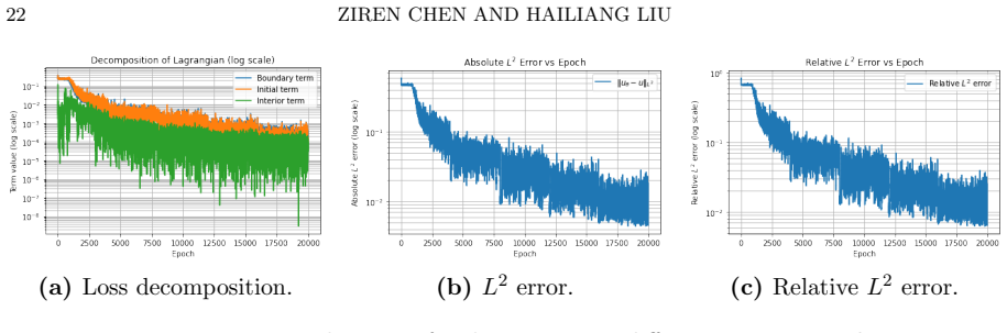
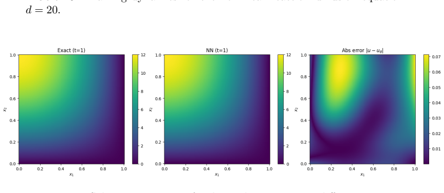
Summary. The paper extends InfSupNet to a broader class of PDEs by reformulating (1.1) as a constrained minimization (1.2) and then as an inf-sup problem (1.3) via a Lagrange multiplier. Theorems 1–2 establish equivalence of the continuous formulations under well-posedness. Two networks parameterize the primal and dual variables and are trained by alternating GDA (Algorithm 1). For linear well-posed problems the residual-controlled stability estimate (4.1)–(4.2) yields the three-term error bound of Theorems 3–4; for linear convection–diffusion under a reduced L^{2} loss the authors further bound I_NN and I_MC explicitly (Theorem 6), leaving I_GP as an optimization residual. Numerical experiments on linear convection–diffusion (d=3,5) and several nonlinear problems (reaction–diffusion up to d=20, Burgers, Allen–Cahn) report relative L^{2} errors of order 10^{-3}.
Significance. The work supplies a clean residual-to-error decomposition for linear PDEs that simultaneously controls the primal solution and the dual multiplier, together with a practical reduced-regularity loss that avoids high-order boundary norms. The continuous equivalence proofs (Theorems 1–2) and the Monte-Carlo / fractional-Sobolev sampling analysis feeding Theorem 6 are carefully tracked. If the optimization gap can be controlled, the framework would give a transparent a-posteriori certificate for neural PDE solvers in high dimensions. The nonlinear experiments, while outside the theory, indicate that the same architecture remains stable on stiff and high-dimensional problems.
major comments (3)
- The central quantitative claim (Theorems 3–6) is ∥u_n−u∥^{2}_X + ∥v_n∥^{2}_{Z*} ≤ C(I_NN + I_MC + I_GP). I_GP is defined exactly as the empirical saddle gap at the trained pair (u_n,v_n). Remark 2 states that this gap is uncontrolled for general nonconvex–nonconcave GDA, and the numerical sections never report its magnitude. Consequently the bound does not yet guarantee that the trained network is close to the PDE solution; it only absorbs residual error into an unestimated term. Either a concrete bound (or decay plot) for I_GP under the stated assumptions, or a clear statement that the result is conditional on I_GP o0, is needed for the claim to be load-bearing.
- Section 4.1 and the proofs of Theorems 3–4 rely on linearity of F and B so that the residual of e=u_n−u is exactly F[e] and Be. Remark 4 and Subsections 6.2–6.4 present nonlinear experiments (reaction–diffusion, Burgers, Allen–Cahn) without corresponding theory. The abstract and contribution list should explicitly restrict the error analysis to linear problems and label the nonlinear results as empirical only, so that the scope of the theorems is not overstated.
- Theorem 6 (and Remark 1) assumes that the parameter spaces of U_θ and V_τ remain uniformly bounded so that the constants C_u, C_v, C_1–C_4 stay finite as n o∞. No mechanism (weight clipping, regularization, or a-posteriori check) is provided to enforce this hypothesis during training. Without it the almost-sure bound (5.4) is not guaranteed for the iterates actually produced by Algorithm 1.
minor comments (4)
- Typographical slips: “minimizaiton” (p. 4), “sovles” (p. 11), “hlaved” (p. 21), “inreqased” (p. 26), “Owning to” (p. 29).
- Figure 5 captions list “Dimension d=1,…,5” but the corresponding panel is not fully described in the text; a short legend clarifying the plotted quantity would help.
- The dual-network L^{2}-norm plot (Figure 6) is shown only for d=3; a brief remark on its behaviour for the higher-dimensional or nonlinear cases would strengthen the saddle-point interpretation.
- References [16] and [32] are central; a one-sentence comparison of the present error decomposition with the elliptic analysis of [16] would clarify the incremental contribution.
Circularity Check
Minor non-load-bearing self-citation to prior InfSupNet [16]; equivalence proofs and residual-stability error decomposition are self-contained and not forced by definition or fit.
specific steps
-
self citation load bearing
[Section 1 (Related work / Main contributions) and opening of Section 4]
"Building on this perspective, the present work develops a more general inf–sup neural framework... building on the framework of [16], we establish error bounds for linear well-posed PDEs... The present analysis can be viewed as a natural extension of this framework."
The method and error-decomposition strategy are presented as an extension of the authors' own prior InfSupNet paper [16]. This is ordinary self-citation of a foundational special case; it is not load-bearing because Theorems 1–2 and the residual-stability argument of Theorem 3 are proved from scratch without relying on unverified claims from [16].
full rationale
The paper's core claims (Theorems 1–2 equivalence of PDE / constrained / inf-sup; Theorems 3–6 residual-controlled error split into I_NN + I_MC + I_GP for linear well-posed problems, with explicit Monte-Carlo and approximation rates for convection–diffusion under reduced L2 loss) are derived from first principles inside the manuscript: well-posedness + Riesz map rewriting of residual norms + best-approximation projections onto network classes + standard MC concentration. The three-term bound is a transparent a-posteriori decomposition, not a tautology that assumes the conclusion; I_GP is left explicitly uncontrolled (Remark 2) rather than claimed small by construction. Self-citation to the authors' earlier InfSupNet [16] appears for the elliptic special case and the overall saddle-point idea, but the new parabolic analysis, reduced-regularity loss (4.20), and proofs do not reduce to that citation. No fitted parameters are re-labeled as predictions, no uniqueness theorem is imported to forbid alternatives, and no ansatz is smuggled. Nonlinear experiments lie outside the linear theory (as the paper itself notes) but do not create circularity. Score 2 reflects only the non-load-bearing self-citation; the derivation chain is otherwise independent.
Axiom & Free-Parameter Ledger
free parameters (4)
- Network depth and width (primal and dual)
- Interior/boundary/initial sample counts (m, m0, m̂, n̂)
- Ascent/descent steps k,l and learning rates η_θ, η_τ with decay
- Training epoch budgets
axioms (7)
- domain assumption The PDE (1.1) is well-posed with unique solution in the chosen Banach/Hilbert spaces.
- domain assumption Linear stability: ∥u∥_X² ≤ C(∥f∥_Z² + ∥g∥_P²) (and the reduced-regularity L2 version for parabolic problems).
- domain assumption F and B are linear for the error analysis.
- standard math Neural networks in U_θ, V_τ can approximate the required Sobolev/space-time targets (with C^{max(p,s)} activations for the primal).
- standard math Monte Carlo and tensor-product fractional-Sobolev quadrature error rates as in [5,6].
- ad hoc to paper Parameter spaces of U_θ and V_τ remain uniformly bounded so error constants stay finite as n→∞.
- ad hoc to paper Saddle-point training makes the optimization gap I_GP small under suitable structural assumptions.
invented entities (1)
-
InfsupNet / dual Lagrange-multiplier network v_τ
no independent evidence
Cite this review
Pith. "Pith review of Inf-Sup Neural Networks for High Dimensional PDEs." pith.science (2026). https://pith.science/paper/GA2CAYBD
@misc{pith2026260711718,
  author       = {Pith},
  title        = {Pith review of: Inf-Sup Neural Networks for High Dimensional PDEs},
  year         = {2026},
  howpublished = {\url{https://pith.science/paper/GA2CAYBD}},
  note         = {Machine review of arXiv:2607.11718}
}
read the original abstract
Solving partial differential equations (PDEs) in high dimensions remains challenging due to the curse of dimensionality. We propose a neural-network-based framework that reformulates PDEs as inf--sup optimization problems through the introduction of a Lagrange multiplier. The primal solution and the associated Lagrange multiplier are parameterized by two networks and are computed via an iterative saddle-point optimization procedure. We prove the theoretical equivalence between the proposed optimization formulation and the original PDE problem, and we derive rigorous error estimates that quantify the total approximation error in terms of the network approximation error, statistical (sampling) error, and optimization error. Numerical experiments demonstrate the accuracy, stability, and efficiency of the proposed method for solving high-dimensional PDEs.
Figures




Reference graph
Works this paper leans on
-
[1]
3, 499–541
Ahmed Abdeljawad and Philipp Grohs,Approximations with deep neural networks in Sobolev time- space, Analysis and Applications20(2022), no. 3, 499–541
2022
-
[2]
David Alvarez-Melis, Yair Schiff, and Youssef Mroueh,Optimizing functionals on the space of prob- abilities with input convex neural networks, Transactions on Machine Learning Research (2022)
2022
-
[3]
6, C688–C715
Silvia Bertoluzza, Erik Burman, and Cuiyu He,WAN discretization of PDEs: Best approximation, stabilization, and essential boundary conditions, SIAM Journal on Scientific Computing46(2024), no. 6, C688–C715
2024
-
[4]
Boffi and Eric Vanden-Eijnden,Probability flow solution of the Fokker–Planck equation, Machine Learning: Science and Technology4(2023), no
Nicholas M. Boffi and Eric Vanden-Eijnden,Probability flow solution of the Fokker–Planck equation, Machine Learning: Science and Technology4(2023), no. 3, 035012
2023
-
[5]
Siegel,Convergence and error control of consistent PINNs for elliptic PDEs, IMA Journal of Numerical Analysis46(2025), no
Andrea Bonito, Ronald DeVore, Guergana Petrova, and Jonathan W. Siegel,Convergence and error control of consistent PINNs for elliptic PDEs, IMA Journal of Numerical Analysis46(2025), no. 1, 90–148
2025
-
[6]
Caflisch,Monte Carlo and quasi-Monte Carlo methods, Acta Numerica7(1998), 1–49
Russel E. Caflisch,Monte Carlo and quasi-Monte Carlo methods, Acta Numerica7(1998), 1–49
1998
-
[7]
4, 303–314
George Cybenko,Approximation by superpositions of a sigmoidal function, Mathematics of Control, Signals and Systems2(1989), no. 4, 303–314
1989
-
[8]
Tim De Ryck, Samuel Lanthaler, and Siddhartha Mishra,On the approximation of functions by tanh neural networks, Neural Networks143(2021), 732–750
2021
-
[9]
Tim De Ryck and Siddhartha Mishra,Error analysis for physics-informed neural networks (PINNs) approximating kolmogorov PDEs, Advances in Computational Mathematics48(2022), no. 6, 79
2022
-
[10]
2, 811–841
Tim De Ryck, Siddhartha Mishra, and Roberto Molinaro,wPINNs: Weak physics-informed neural networks for approximating entropy solutions of hyperbolic conservation laws, SIAM Journal on Numerical Analysis62(2024), no. 2, 811–841
2024
-
[11]
3, 195– 201
Gamini Dissanayake and Nhan Phan-Thien,Neural-network-based approximations for solving partial differential equations, Communications in Numerical Methods in Engineering10(1994), no. 3, 195– 201
1994
-
[12]
Weinan E and Bing Yu,The deep Ritz method: A deep learning-based numerical algorithm for solving variational problems, Communications in Mathematics and Statistics6(2018), no. 1, 1–12
2018
-
[13]
6185–6215
Jiaojiao Fan, Qinsheng Zhang, Amirhossein Taghvaei, and Yongxin Chen,Variational Wasserstein gradient flow, Proceedings of the 39th International Conference on Machine Learning, PMLR, 2022, pp. 6185–6215
2022
-
[14]
32 ZIREN CHEN AND HAILIANG LIU
Tianhao Hu, Bangti Jin, and Fengru Wang,An iterative deep Ritz method for monotone elliptic problems, Journal of Computational Physics527(2025), 113791. 32 ZIREN CHEN AND HAILIANG LIU
2025
-
[15]
Karniadakis, and Kenji Kawaguchi,Score-based physics- informed neural networks for high-dimensional Fokker–Planck equations, SIAM Journal on Scientific Computing47(2025), no
Zheyuan Hu, Zhongqiang Zhang, George E. Karniadakis, and Kenji Kawaguchi,Score-based physics- informed neural networks for high-dimensional Fokker–Planck equations, SIAM Journal on Scientific Computing47(2025), no. 3, C680–C705
2025
-
[16]
Xiaokai Huo and Hailiang Liu,Inf-sup neural networks for high-dimensional elliptic PDE problems, Journal of Computational Physics514(2024), 113188
2024
-
[17]
Jagtap and George E
Ameya D. Jagtap and George E. Karniadakis,Extended physics-informed neural networks (XPINNs): A generalized space-time domain decomposition framework for nonlinear partial differential equa- tions, Communications in Computational Physics28(2020), no. 5, 2002–2041
2020
-
[18]
Yuling Jiao, Yanming Lai, Yang Wang, Haizhao Yang, and Yunfei Yang,Convergence analysis of the deep Galerkin method for weak solutions, From Classical Analysis to Analysis on Fractals: A Tribute to Robert Strichartz, Volume 1, Springer International Publishing, Cham, 2023, pp. 53–82
2023
-
[19]
4880–4889
Chi Jin, Praneeth Netrapalli, and Michael Jordan,What is local optimality in nonconvex-nonconcave minimax optimization?, Proceedings of the 37th International Conference on Machine Learning, PMLR, 2020, pp. 4880–4889
2020
-
[20]
Richard Jordan, David Kinderlehrer, and Felix Otto,The variational formulation of the Fokker– Planck equation, SIAM Journal on Mathematical Analysis29(1998), no. 1, 1–17
1998
-
[21]
Karniadakis,Variational physics-informed neu- ral networks for solving partial differential equations, 2019
Ehsan Kharazmi, Zhongqiang Zhang, and George E. Karniadakis,Variational physics-informed neu- ral networks for solving partial differential equations, 2019
2019
-
[22]
Mahoney,Charac- terizing possible failure modes in physics-informed neural networks, Advances in Neural Information Processing Systems, vol
Aditi Krishnapriyan, Amir Gholami, Shandian Zhe, Robert Kirby, and Michael W. Mahoney,Charac- terizing possible failure modes in physics-informed neural networks, Advances in Neural Information Processing Systems, vol. 34, 2021, pp. 26548–26560
2021
-
[23]
Lagaris, Aristidis Likas, and Dimitrios I
Isaac E. Lagaris, Aristidis Likas, and Dimitrios I. Fotiadis,Artificial neural networks for solving ordinary and partial differential equations, IEEE Transactions on Neural Networks9(1998), no. 5, 987–1000
1998
-
[24]
Lingxiao Li, Samuel Hurault, and Justin Solomon,Self-consistent velocity matching of probability flows, Advances in Neural Information Processing Systems36(2023), 57038–57057
2023
-
[25]
Shaofan Li and Wing Kam Liu,Meshfree and particle methods and their applications, Applied Me- chanics Reviews55(2002), no. 1, 1–34
2002
-
[26]
Wuchen Li, Shu Liu, Hongyuan Zha, and Haomin Zhou,Parametric Fokker–Planck equation, Geo- metric Science of Information: 4th International Conference, GSI 2019 (Cham), Springer, 2019, pp. 715–724
2019
-
[27]
Zongyi Li, Nikola Kovachki, Kamyar Azizzadenesheli, Burigede Liu, Kaushik Bhattacharya, and Andrew Stuart,Fourier neural operator for parametric partial differential equations, arXiv preprint arXiv:2010.08895 (2021)
Pith/arXiv arXiv 2010
-
[28]
6083–6093
Tianyi Lin, Chi Jin, and Michael Jordan,On gradient descent ascent for nonconvex-concave minimax problems, Proceedings of the 37th International Conference on Machine Learning, PMLR, 2020, pp. 6083–6093
2020
-
[29]
Jacques-Louis Lions and Enrico Magenes,Non-homogeneous boundary value problems and applica- tions, Springer, 1972
1972
-
[30]
Min Liu, Zhiqiang Cai, and Karthik Ramani,Deep Ritz method with adaptive quadrature for linear elasticity, Computer Methods in Applied Mechanics and Engineering415(2023), 116229
2023
-
[31]
3, 1385–1449
Shu Liu, Wuchen Li, Hongyuan Zha, and Haomin Zhou,Neural parametric Fokker–Planck equation, SIAM Journal on Numerical Analysis60(2022), no. 3, 1385–1449
2022
-
[32]
Shu Liu, Stanley Osher, and Wuchen Li,A natural primal-dual hybrid gradient method for adversarial neural network training on solving partial differential equations, 2024, arXiv:2411.06278
Pith/arXiv arXiv 2024
-
[33]
Jianfeng Lu, Yue Wu, and Yang Xiang,Score-based transport modeling for mean-field Fokker–Planck equations, Journal of Computational Physics503(2024), 112859
2024
-
[34]
Karniadakis,Learning non- linear operators via DeepONet based on the universal approximation theorem of operators, Nature Machine Intelligence3(2021), no
Lu Lu, Pengzhan Jin, Guofei Pang, Zhongqiang Zhang, and George E. Karniadakis,Learning non- linear operators via DeepONet based on the universal approximation theorem of operators, Nature Machine Intelligence3(2021), no. 3, 218–229
2021
-
[35]
3196–3241
Yulong Lu, Jianfeng Lu, and Min Wang,A priori generalization analysis of the deep Ritz method for solving high dimensional elliptic partial differential equations, Proceedings of the Thirty Fourth Conference on Learning Theory, 2021, pp. 3196–3241. INF–SUP 33
2021
-
[36]
McClenny and Ulisses M
Levi D. McClenny and Ulisses M. Braga-Neto,Self-adaptive physics-informed neural networks, Jour- nal of Computational Physics474(2023), 111722
2023
-
[37]
Ensela Mema, Ting Wang, and Jaroslaw Knap,Deep Ritz method with Fourier feature mapping: A deep learning approach for solving variational models of microstructure, Journal of Computational Science91(2025), 102631
2025
-
[38]
Piotr Minakowski and Thomas Richter,A priori and a posteriori error estimates for the deep Ritz method applied to the Laplace and Stokes problem, Journal of Computational and Applied Mathe- matics421(2023), 114845
2023
-
[39]
Shiv Mishra and Arbaz Khan,A priori error analysis of consistent PINNs for parabolic PDEs, 2025, arXiv:2506.17614
Pith/arXiv arXiv 2025
-
[40]
Siddhartha Mishra and Roberto Molinaro,Estimates on the generalization error of physics-informed neural networks for approximating PDEs, IMA Journal of Numerical Analysis43(2023), no. 1, 1–43
2023
-
[41]
34, 2021, pp
Petr Mokrov, Alexander Korotin, Lingxiao Li, Aude Genevay, Justin Solomon, and Evgeny Burnaev, Large-scale Wasserstein gradient flows, Advances in Neural Information Processing Systems, vol. 34, 2021, pp. 15243–15256
2021
-
[42]
1, 229–251
Arkadi Nemirovski,Prox-method with rate of convergenceO(1/t)for variational inequalities with lipschitz continuous monotone operators and smooth convex-concave saddle point problems, SIAM Journal on Optimization15(2004), no. 1, 229–251
2004
-
[43]
Maher Nouiehed, Maziar Sanjabi, Tianjian Huang, Jason D. Lee, and Meisam Razaviyayn,Solv- ing a class of non-convex min-max games using iterative first order methods, Advances in Neural Information Processing Systems, Curran Associates, Inc., 2019, pp. 14934–14942
2019
-
[44]
Maziar Raissi, Paris Perdikaris, and George E. Karniadakis,Physics-informed neural networks: A deep learning framework for solving forward and inverse problems involving nonlinear partial differ- ential equations, Journal of Computational Physics378(2019), 686–707
2019
-
[45]
5, 55–66
Meisam Razaviyayn, Tianjian Huang, Songtao Lu, Maher Nouiehed, Maziar Sanjabi, and Mingyi Hong,Nonconvex min-max optimization: Applications, challenges, and recent theoretical advances, IEEE Signal Processing Magazine37(2020), no. 5, 55–66
2020
-
[46]
Martin Schechter,OnL p estimates and regularity II, Mathematica Scandinavica13(1963), 47–69
1963
-
[47]
36, 2023, pp
Zebang Shen and Zhenfu Wang,Entropy-dissipation informed neural network for McKean–Vlasov type PDEs, Advances in Neural Information Processing Systems, vol. 36, 2023, pp. 59227–59238
2023
-
[48]
Zebang Shen, Zhenfu Wang, Satyen Kale, Alejandro Ribeiro, Amin Karbasi, and Hamed Hassani, Self-consistency of the Fokker–Planck equation, Proceedings of the Thirty Fifth Conference on Learn- ing Theory, PMLR, 2022, pp. 817–841
2022
-
[49]
Justin Sirignano and Konstantinos Spiliopoulos,DGM: A deep learning algorithm for solving partial differential equations, Journal of Computational Physics375(2018), 1339–1364
2018
-
[50]
4, 507–554
Eitan Tadmor,A review of numerical methods for nonlinear partial differential equations, Bulletin of the American Mathematical Society49(2012), no. 4, 507–554
2012
-
[51]
Tijmen Tieleman and Geoffrey Hinton,Lecture 6.5—RMSProp: Divide the gradient by a running average of its recent magnitude, COURSERA: Neural Networks for Machine Learning, 2012
2012
-
[52]
Sifan Wang and Paris Perdikaris,Long-time integration of parametric evolution equations with physics-informed DeepONets, Journal of Computational Physics475(2023), 111855
2023
-
[53]
5, A3055–A3081
Sifan Wang, Yujun Teng, and Paris Perdikaris,Understanding and mitigating gradient flow patholo- gies in physics-informed neural networks, SIAM Journal on Scientific Computing43(2021), no. 5, A3055–A3081
2021
-
[54]
40, eabi8605
Sifan Wang, Hanwen Wang, and Paris Perdikaris,Learning the solution operator of parametric partial differential equations with physics-informed DeepONets, Science Advances7(2021), no. 40, eabi8605
2021
-
[55]
Sifan Wang, Xinling Yu, and Paris Perdikaris,When and why PINNs fail to train: A neural tangent kernel perspective, Journal of Computational Physics449(2022), 110768
2022
-
[56]
1, 360–395
Hao Wu, Shu Liu, Xiaojing Ye, and Haomin Zhou,Parameterized Wasserstein Hamiltonian flow, SIAM Journal on Numerical Analysis63(2025), no. 1, 360–395
2025
-
[57]
9, 10629–10636
Wuzhe Xu, Yulong Lu, and Li Wang,Transfer learning enhanced DeepONet for long-time prediction of evolution equations, Proceedings of the AAAI Conference on Artificial Intelligence37(2023), no. 9, 10629–10636. 34 ZIREN CHEN AND HAILIANG LIU
2023
-
[58]
Karniadakis,Gradient-enhanced physics-informed neural networks for forward and inverse PDE problems, Computer Methods in Applied Mechanics and Engineering393(2022), 114823
Jeremy Yu, Lu Lu, Xuhui Meng, and George E. Karniadakis,Gradient-enhanced physics-informed neural networks for forward and inverse PDE problems, Computer Methods in Applied Mechanics and Engineering393(2022), 114823
2022
-
[59]
Yaohua Zang, Gang Bao, Xiaojing Ye, and Haomin Zhou,Weak adversarial networks for high- dimensional partial differential equations, Journal of Computational Physics411(2020), 109409
2020
-
[60]
Mo Zhou, Stanley Osher, and Wuchen Li,Score-based neural ordinary differential equations for computing mean field control problems, Journal of Computational Physics542(2025), 114369
2025
-
[61]
,Simulating Fokker–Planck equations via mean field control of score-based normalizing flows, 2025, arXiv:2506.05723
Pith/arXiv arXiv 2025
-
[62]
Qijia Zhou, Yiyang Wang, Shengyuan Deng, and Chenliang Li,Deep Ritz physics-informed neural network method for solving the variational inequality problems, IAENG International Journal of Applied Mathematics55(2025), no. 12. AppendixA.Proof of Lemma 5 Proof.We employ the method of transposition. Letψ∈L 2(ΩT ) be an arbitrary test function. Consider the bac...
2025
This paper was first reviewed by grok-4.5 on July 14, 2026.
discussion (0)
Sign in with ORCID, Apple, or X to comment. Anyone can read and Pith papers without signing in.