Bridging Frustration and Non-Hermiticity via COMPASS: An Adaptive Biorthogonal Neural Quantum State Framework

Flore K. Kunst; Lavoisier Wah; Mohamed Hibat-Allah

REVIEW 4 major objections 6 minor 57 references

Bridging Frustration and Non-Hermiticity via COMPASS: An Adaptive Biorthogonal Neural Quantum State Framework

T0 review · 4 major / 6 minor · reviewed 2026-08-02 · deepseek-v4-flash

Challenge this review Re-run · record.json Download PDF Read on arXiv ↗

Pith's one-line read This paper introduces COMPASS, a biorthogonal adaptive neural-network method that simulates non-Hermitian many-body systems directly and reveals that frustration gaps shield spectra from non-Hermitian instability while complex couplings cre

desk verdict Useful ansatz-selection insight and credible ED-scaled observations, but the convergence guarantee underpinning the large-N claims is asserted, not proven. read the letter →

arxiv 2607.13790 v1 pith:OTLYJXVW submitted 2026-07-15 quant-ph

Lavoisier Wah , Flore K. Kunst , Mohamed Hibat-Allah This is my paper

classification quant-ph

keywords non-HermitianquantumsystemsneuralstatesbiorthogonalvariationalMonteCarloparity-timesymmetryfrustratedmagnetismdiabolicringadaptiverecurrentnetworksexceptionalpoints

verification ladder T0 review T1 audit T2 compute T3 formal

The pith

A machine-rendered reading of the paper's core claim, the machinery that carries it, and where it could break.

The reading

COMPASS is a variational framework that lets neural quantum states tackle non-Hermitian many-body systems directly, without mapping them onto Hermitian problems or slowly switching on non-Hermiticity. The paper shows that the choice of ansatz is physically decisive: for parity-time-symmetric Hamiltonians, an unconstrained complex neural network can spontaneously break the symmetry and produce spurious imaginary energies, while a real-valued network stays on the physical manifold; for generic non-Hermitian Hamiltonians the reverse is true. With the framework the authors simulate frustrated spin chains and find that the energy gap from frustration protects the spectrum against non-Hermitian instability up to a critical strength, and that making the frustration coupling complex produces a closed ring of level crossings—the 'diabolic ring'—a spectral topology with no Hermitian counterpart. If correct, this opens non-Hermitian frustrated magnets to scalable numerical study and suggests that symmetry-aware architecture choice, not raw expressivity, is what makes variational simulations reliable.

What carries the argument

The central machinery is COMPASS: a pair of independent gated-recurrent-unit autoregressive neural networks, one for the right eigenstate and one for the left, whose log-amplitudes are complex and factorized as products of conditionals with probability and phase parts. It combines biorthogonal variational Monte Carlo (sampling from |Ψ_L Ψ_R|) with a complementary loss L = λ_t L_e + (1-λ_t)L_v that alternates energy minimization (to select the ground state) and variance minimization (to enforce the eigenstate condition), plus a warm-start schedule and an adaptive architecture that grows the hidden dimension while transferring parameters. Exact autoregressive sampling removes Markov-chain nois

What would settle it

Exact-diagonalize a small (N≤12) instance of the complex-NNN J1-J2 model and run COMPASS from many random initializations: if any run converges to a zero-variance pair whose real-part energy exceeds the exact ground-state energy, the complementary-loss convergence claim fails. A second, independent test: measure the maximum eigenvector overlap at a point on the diabolic ring—if the overlap approaches 1, the ring is exceptional, not diabolic.

Watch

Extended reading notes

Core claim

The paper's central claim is that a biorthogonal adaptive neural-network ansatz—two independent autoregressive recurrent networks representing the left and right eigenstates, trained with a complementary loss that alternates energy and variance minimization—converges to the correct ground-state eigenpair of a generic non-Hermitian Hamiltonian, enabling direct simulation of 1D (up to N=200) and 2D (up to N=100) systems without Hermitian embeddings or adiabatic continuation. Alongside the method, the paper establishes two physical results: (i) in PT-symmetric systems, real-valued ansätze are necessary to avoid spurious spontaneous PT breaking during optimization, while complex ansätze are esse

Load-bearing premise

The load-bearing premise is that minimizing the complementary loss (sum of energy and variance) reliably lands on the smallest-real-part biorthogonal eigenpair; the paper asserts this convergence but offers no proof that the energy loss of the pure left and right expectations selects the biorthogonal ground state rather than some other eigenpair.

Editorial extensions

If this is right

Ansatz selection is physically decisive: real-valued networks are required for PT-symmetric models to avoid spurious imaginary energies; complex networks are required for generic non-Hermitian spectra.
The frustration gap Δ sets the critical threshold for PT-symmetry breaking, γ_c ∝ Δ, so frustrated gapped phases are quantitatively shielded against non-Hermitian spectral instability.
Complexifying the frustration coupling yields a closed diabolic ring of real-energy level crossings with eigenvalue braiding, a spectral topology with no Hermitian analog and controlled by the phase of the complex coupling, not its modulus.
Direct simulation of non-Hermitian many-body systems is possible up to N=200 (1D) and N=100 (2D) without Hermitian embeddings or adiabatic continuation, with high biorthogonal fidelity.
The 'effective frustration' hypothesis (replacing the complex coupling by its modulus) is disproved by the absence of a phase transition along the predicted quarter-circle locus.

Reading between the lines

Editorial extensions of the paper, not claims the author makes directly.

We infer that if the convergence guarantee holds, COMPASS should generalize to time-dependent non-Hermitian dynamics and to higher-dimensional frustrated lattices, where the diabolic ring might become a surface or higher-dimensional crossing manifold.
We infer that the ansatz-selection principle—constraining the network to the symmetry class of the target state beats unconstrained expressivity—likely extends to other variational families and could be formalized as a bias-variance trade-off specific to non-Hermitian optimization landscapes.
If the diabolic ring is robust to finite-size effects, it offers a testable signature of non-Hermitian frustration in cold-atom or trapped-ion simulators, where the complex next-nearest-neighbor coupling could be engineered via lossy intermediate sites.
The real part of the biorthogonal variance, which the paper notes changes sign at the PT transition, could serve as a cheap numerical order parameter for locating exceptional points in larger systems.

Share X Bluesky LinkedIn Reddit HN

Editorial analysis

A structured set of objections, weighed in public.

Desk editor's note, referee report, and a circularity audit.

Desk Editor's Note

read the letter

Colleague — quick take: the paper is worth reading for two things: the observation that complex-valued RNN ansätze spontaneously break PT symmetry during optimization in the unbroken phase, and the ED-backed finding that a frustration gap shields PT symmetry with γ_c ∝ Δ. The larger claim — COMPASS reaches N=200/100 without Hermitian embeddings or adiabatic continuation — is plausible but not actually established.

What’s new and good: the package of adaptive RNN growth, independent left/right biorthogonal networks, exact autoregressive sampling, and alternating energy/variance minimization is a real methodological contribution. The ansatz-selection result is non-obvious and useful: a real ansatz constrains the optimization to the real-spectrum manifold for PT-symmetric systems, while complex ansätze are needed for generic complex spectra. The gap-frustration shield is a parameter-free ED observation with stated assumptions; the phase diagrams in Figs. 7–8 look consistent with that narrative. The diabolic ring is an interesting level-crossing locus, though I’d call it “observed” rather than “topologically nontrivial” without a formal braiding analysis — the authors themselves note no EPs are detected and leave eigenvalue tracking for larger γ.

The soft spot is load-bearing. Section II.A.4 and Appendix B define the energy loss as a sum of pure left/right expectations (Eq. B2), not the biorthogonal mixed estimator. For non-Hermitian H these pure expectations have no variational lower bound and are generally complex. The paper asserts that the complementary loss “ensures” convergence to the ground-state biorthogonal pair, but no stationary-point argument or counterexample shows that minimizing this sum selects the smallest-real-part pair. The variance term only forces each state to be an eigenstate of H (right) and H† (left) with a common eigenvalue; it doesn’t select the ground state. The warm-start protocol is heuristic, and Appendix C shows pure variance can land on excited states. Since ED benchmarks stop at N=10–14, the N=200 (1D) and N=100 (2D) claims and the large-N phase diagrams inherit this unverified assumption. The N=10 ED agreement in Fig. 10 is real supporting evidence, but it doesn’t cover the regime where the strongest scalability claims are made. Minor issues: Fig. 4 has a literal missing parameter (δλ=?), and the code is under embargo despite the data availability statement.

Overall: this is a serious piece of work with credible small-system results and an honest tendency to report its own failed predictions — the effective-frustration hypothesis is explicitly falsified in the text. I’d send it to peer review with a request for substantial revision, not desk reject. The referee should ask for a proof or at least a counterexample-based argument for convergence of Eq. B2, a clear statement of what the large-N results actually validate, and a more careful topological characterization of the diabolic ring.

Referee Report

4 major / 6 minor

Summary. The paper introduces COMPASS, a non-Hermitian neural quantum state method built from two adaptive recurrent networks representing left and right eigenstates, trained with a complementary loss (Eq. 8) that switches between energy minimization and variance minimization, with exact autoregressive sampling rather than MCMC. The authors demonstrate the method on 1D and 2D PT-symmetric transverse-field Ising chains, report adaptive/static speed comparisons, and argue that real-valued ansätze are necessary in the PT-unbroken phase while complex ansätze are needed for generic complex spectra. They then study two non-Hermitian J1-J2 spin-chain models: one with a staggered imaginary field (Model 1) and one with a complex next-nearest-neighbor coupling (Model 2). For Model 1 they claim a 'frustration-gap shield' whereby the spectral gap sets a quantitative threshold for PT breaking; for Model 2 they claim a 'diabolic ring'—a closed curve of real-part level crossings with no Hermitian analog, associated with eigenvalue braiding. Large-system claims are made for N=200 (1D) and N=100 (2D) TFIM simulations, while the frustrated models are benchmarked only at N=10 against exact diagonalization.

Significance. If the convergence and topology claims hold, COMPASS would be a genuinely useful extension of neural quantum states to non-Hermitian, frustrated and non-stoquastic systems, and the ansatz-selection insight (real vs complex networks) is physically well motivated. The paper's strengths include exact autoregressive sampling without MCMC, a clean adaptive capacity schedule, explicit ED benchmarks at N=10, and an honest self-falsification of the naive |J2+iγ| effective-coupling hypothesis in Sec. V.B. However, the advertised guarantees are currently stronger than what is demonstrated: the complementary loss has no proven ground-state selection property, the diabolic-ring braiding is asserted rather than computed, and the 'quantitative' gap-shield relation is not backed by scaling data. These issues are load-bearing for the central claims, so a major revision is required.

major comments (4)

[Sec. II.A.4 / App. B / App. C] The statement that the complementary loss 'ensures' convergence to the correct ground-state biorthogonal pair is not derived. With Eq. (B2), L_e = ⟨ΨR|H|ΨR⟩/⟨ΨR|ΨR⟩ + ⟨ΨL|H†|ΨL⟩/⟨ΨL|ΨL⟩, the energy loss is a sum of pure left/right expectations, not the mixed biorthogonal estimator of Eq. (2). For non-Hermitian H these expectations have no variational lower bound and are generally complex; the text does not specify how a complex loss is optimized. The variance terms force |ΨR⟩ and |ΨL⟩ to be eigenstates of H and H† with a common eigenvalue but do not select the ground state, and the λ_t warm-start schedule is heuristic. Appendix C benchmarks against ED only at N=10 for the PT-symmetric TFIM; the large-N comparisons use SE, not an independent NH solver. Since the N=200/100 claims and the frustrated-model results inherit this assumption, please provide a stationary-point argument for Eq. (8
[Sec. V.C / Fig. 9] The central new-topology claim—the 'diabolic ring' supporting eigenvalue braiding—is not demonstrated. The ring is identified as the locus where Re(E1)=Re(E0) with distinct imaginary parts, i.e., a real-part degeneracy line. The paper asserts that encircling the ring exchanges E0 and E1 ('spectral flow topology'), but no closed loop in (J2,γ) is tracked, no eigenvector-following or monodromy calculation is shown, and no braid invariant is computed. The maximum eigenvector overlap of ≈0.89 reported in Appendix I does not establish the absence of EPs by itself. Without this evidence, the ring is an interesting level-crossing curve, but the 'topologically nontrivial' and 'no Hermitian analog' statements are unsupported. Please provide the braiding/monodromy data or substantially qualify the claim.
[Sec. V.B / Figs. 7-8] The 'quantitative shield' relation γ_c ∝ Δ is not supported by the displayed data. At the Majumdar-Ghosh point (J2/J1=0.5), the zero-field gap within the Sz=0 sector is exactly zero (Fig. 7c), yet Fig. 8a shows |Im E0|=0 up to γ_c≈0.95. Thus the threshold is not set by the zero-field gap; at the MG point the protection must instead arise from the γ-induced splitting of the degenerate dimer states. A plot of γ_c versus the relevant gap, or a finite-size scaling analysis, is needed before calling the shield quantitative. As written, the mechanism is plausible but the quantitative claim is unjustified.
[Secs. III-V / Abstract] The large-scale demonstrations (N=200 in 1D, N=100 in 2D) are only for the PT-symmetric TFIM, where the spectrum is real in the unbroken phase and the model is stoquastic-like. The frustrated J1-J2 models, which are the basis for the 'beyond stoquasticity' and 'direct study of NH many-body systems' claims, are benchmarked only at N=10 against ED. The abstract and conclusion should either distinguish 'method scales on the TFIM' from 'method works for frustrated NH systems' or include a large-N frustrated benchmark. This is not a fatal flaw, but it currently overstates the scope of the numerical evidence.

minor comments (6)

[Fig. 4 caption] The caption contains 'δλ=?' with no value or definition; this should be specified.
[Appendix B, Eq. (B4)] The left/right variance losses are labeled L_R^e and L_L^e; these should be L_R^v and L_L^v to match Eq. (B3).
[Table I / Sec. III] The abbreviations cRNN, pRNN, and SE are used without explicit definition. 'pRNN' is later described as 'real (positive)', but the relation between 'real-valued' and the amplitude parametrization of Eq. (4) should be clarified.
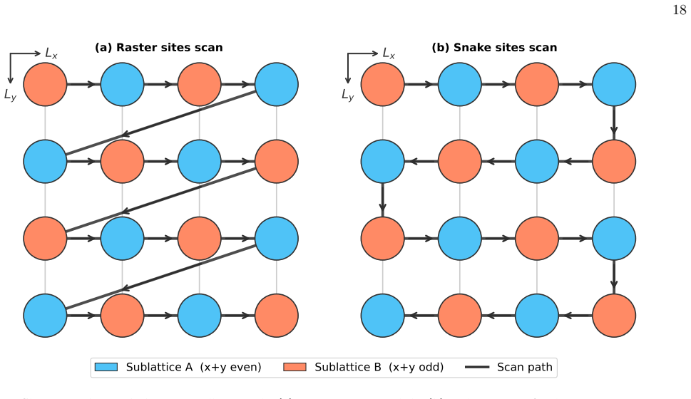
[Sec. IV.B, Fig. 6] The text says the snake scan is 'two orders of magnitude more accurate' but the inset shows ε_rel ≈ 10^-2, i.e., about two orders of magnitude smaller than the raster energy; the phrasing is confusing.
[Sec. V.B and elsewhere] Minor typos: 'bugles outward' should be 'bulges outward'; the Note added contains 'antsatz'; Appendix F has malformed notation 'E ∼ |ΨR|2'.
[Ref. [51]] The GitHub reference lists author names inconsistent with the manuscript author list; please verify the citation entry.

Circularity Check

0 steps flagged · score 1.0 of 10

No significant circularity; the paper's internal predictions are explicitly falsifiable and benchmarked against ED, and the main self-citation is methodological rather than load-bearing.

full rationale

The claimed derivation chain is self-contained in the sense required for evaluating circularity. The only quantities the paper labels as analytical predictions—the ON and MG loci under the effective coupling |J2+iγ|—are stated as assumptions ('We naively predict the ON ... and the MG ... by setting |J2+iγ|≈0.24 and 0.5') and then explicitly tested and disproved against ED ('Neither of the predictions worked'). This is a genuine falsifiable test, not a fit renamed as a prediction. The frustration-gap shield is an ED observation tied to the EP mechanism (γ_c ∝ Δ), not a consequence of a fitted parameter. The diabolic ring is defined as the direct ED locus where Re(E1)=Re(E0); naming this locus is an interpretation, not a derivation from its own definition. The adaptive RNN scheme is taken from Ref. [10], which shares a co-author, but it is described explicitly in the paper (e.g., Eq. (9)) and benchmarked against a static RNN in Table I, so the self-citation is not the sole or unverified support for the paper's conclusions. The convergence claim of the complementary loss is asserted rather than proven—Eq. (B2) is a sum of pure left/right expectations rather than the mixed bVMC estimator, and the paper itself notes limitations and deferred analyses ('we leave such an extension to future work' in Appendix F; 'we limited ourselves to a small system size... leave for future work' in Sec. V.E). That is a correctness risk, not circularity: the final estimator is still benchmarked against independent ED at N=10, and no central result is forced to be true by definition or by an equation that equals its own input. The non-finding is therefore appropriate.

Assumptions & free parameters 5 free parameters · 6 assumptions · 1 invented entities

The method itself introduces several hand-chosen hyperparameters that the convergence claims depend on, but no sensitivity analysis is provided. The main physical results rest on standard ED and the asserted (but unproven) convergence of the complementary loss. The only invented entity is the diabolic ring, for which independent evidence is currently absent.

free parameters (5)

Convergence threshold ε_c = 10^-5
Hand-chosen threshold for switching between energy and variance phases (Sec. II.A.4, Tables II/III); central to warm-start protocol.
Energy weight schedule λ_t = 1 → 0 → 1 (decay rate not specified numerically)
Controls the balance between energy and variance losses (Eq. 8); chosen by hand, no sensitivity analysis.
Warm-up fraction = 0.7 (2D), 0.5 (1D)
Fixes how much of the training budget is pure energy minimization before variance refinement (Tables II/III).
Early stopping patience N_pat = 500-800 steps
Determines when 2D training stops (Appendix D, Table II); hand-chosen.
Adaptive hidden-dimension growth schedule = 2→4→...→128→256
Model capacity schedule from Ref [10]; hand-specified, affects all results.

assumptions (6)

domain assumption Ground state is defined as the eigenstate with smallest real part of the energy.
Stated in Sec. II.A; standard convention in NH quantum mechanics but not universally valid for all purposes.
standard math Biorthogonal VMC with sampling from ρ(x) ∝ |ΨL(x)ΨR(x)| yields unbiased estimators of the mixed expectation.
Appendix A; standard importance-sampling identity.
ad hoc to paper The zero-variance condition σ²_R = ⟨ΨR|(H†−ε*)(H−ε)|ΨR⟩/⟨ΨR|ΨR⟩=0 characterizes eigenpairs, so minimizing variance plus energy converges to the ground-state pair.
The first part is standard; the convergence of the alternating loss (Sec. II.A.4) is asserted without a proof linking pure left/right losses to the biorthogonal ground state.
domain assumption For PT-symmetric Hamiltonians in the unbroken phase, a positive real ansatz in the computational basis can represent the ground state.
Used in Sec. III.C to justify pRNN; no explicit proof that the PT-unbroken ground state is real and nonnegative in the z-basis.
domain assumption The snake scan preserves the sublattice A/B alternation and avoids nonphysical long-range sequential correlations, making it more accurate than raster.
Argued in Sec. IV and Appendix D; supported only by numerical comparison, not by a theorem.
standard math Autoregressive RNN factorization (Eqs. 3-5) is sufficiently expressive to represent left/right eigenstates of NH spin Hamiltonians.
Universal approximation for sequence models; standard NQS assumption.

invented entities (1)

Diabolic ring
purpose: A closed locus in (J2/J1, γ) space where Re(E1)=Re(E0) for the complex-NNN J1-J2 model, proposed as a new NH spectral topology with eigenvalue braiding and no Hermitian analog.
Observed only via ED at N=10 in this paper (Fig. 9, Sec. V.C); no topological invariant is computed and no external falsifiable prediction is made; the maximum eigenvector overlap reaches ~0.89, leaving the distinction from an exceptional ring unproven at larger sizes.

how reviews work

0 comments

Cite this review

Pith. "Pith review of Bridging Frustration and Non-Hermiticity via COMPASS: An Adaptive Biorthogonal Neural Quantum State Framework." pith.science (2026). https://pith.science/paper/OTLYJXVW

@misc{pith2026260713790,
  author       = {Pith},
  title        = {Pith review of: Bridging Frustration and Non-Hermiticity via COMPASS: An Adaptive Biorthogonal Neural Quantum State Framework},
  year         = {2026},
  howpublished = {\url{https://pith.science/paper/OTLYJXVW}},
  note         = {Machine review of arXiv:2607.13790}
}

read the original abstract

In this work, we introduce a complementary optimization method for progressive and adaptive state search (COMPASS) based on biorthogonal adaptive recurrent neural quantum states. Our approach combines an adaptive autoregressive architecture with a biorthogonal variational Monte Carlo scheme as well as a complementary optimization scheme that alternates between energy and variance minimization. This enables the stable convergence to ground-state eigenpairs, while avoiding Markov chain sampling through exact autoregressive generation. We demonstrate that for parity-time(PT)-symmetric Hamiltonians, unconstrained complex ansatze can spontaneously break PT symmetry during optimization, even in the unbroken phase, leading to spurious imaginary energies. Real-valued ansatze, on the other hand, naturally constrain the optimization to the correct physical manifold. Conversely, for generic non-Hermitian (NH) Hamiltonians without symmetry protection and complex spectra, complex ansatze are essential for capturing complex ground-state properties. Our results establish that physically-informed ansatz selection is crucial for reliable NH simulations. By combining adaptive architectures, biorthogonal optimization, and symmetry-aware modeling, this framework enables a direct study of 1D and 2D NH many-body systems without Hermitian embeddings or adiabatic continuation. Applying this framework to systems with frustrated magnetism, we show that gap frustration provides a quantitative shield against NH spectral instability, with the frustration gap setting a critical threshold for PT-symmetry breaking. Also, complexifying the frustration coupling itself generates a new topologically nontrivial network of diabolic level crossings, controlled by the phase of the complex coupling, that has no Hermitian analog. We term this novel spectral topology in NH frustrated systems the diabolic ring.

Figures

Figures reproduced from arXiv: 2607.13790 by the authors.

**Figure 1.** Complementary optimization method for progressive adaptive state search. We show a schematic presentation of our method. (a) We start by building an adaptive RNN, which progressively increases the network capacity during training following an adaptive scheme; then, (b) we initialize two independent RNNs with gated recurrent unit (GRU) cells to represent the right and left eigenstates of the model shown in blue and r… view at source ↗

**Figure 2.** Broken vs unbroken P T symmetry. We plot the imaginary part of the ground-state energy of the 1D Ising chain against its real part for different values of η ∈ [0, 3], and ξ = η/10. We consider δλ = 0.1 + i0.1 when we perturb sublattice A, and δλ = 0.1 − i0.1 when we perturb sublattice B. Open boundries conditions (OBCs) are considered, and N = 10. (TFIM) of N spin-1/2 particles on a lattice subject to a complex stag… view at source ↗

**Figure 3.** Energy per spin for the 1D P T-symmetric Hamiltonian. We plot the imaginary part of the ground-state energy per spin of the 1D P T-symmetric TFIM in Eq. (10), for (a) N = 10, and (b) N = 100 spins using both the adaptive cRNN (in blue) and pRNN (orange). We consider J = 1, η = 1.6 and ξ = 0.16. 0 1000 2000 3000 4000 5000 Training steps 10 1 10 0 0 10 0 10 1 Im(Elo c)/ N Adaptive cRNN Adaptive pRNN (a) 0 1000 2000 30… view at source ↗

Figures from the paper (15 more)

**Figure 4.** Figure 4: Energy per spin for the generic 1D non-Hermitian Hamiltonian. We plot the imaginary part of the ground-state energy per spin of the generic 1D TFIM in Eq. (11), for (a) N = 10, and (b) N = 100 spins using both the adaptive cRNN (in blue) and pRNN (orange). We consider …

**Figure 5.** Figure 5: The 2D P T-symmetric TFIM. We present (a) a schematic representation of the 2D P T-symmetric TFIM (12), and (b) plot the ground state energy per spin with early stopping with the snake scan (blue), and the raster scan (green). We compare the results to ED (black). We c…

**Figure 6.** Figure 6: Final energy for the 2D P T-symmetric TFIM model. We plot the ground state energy of the 2D P T-symmetric TFIM (12) computed after optimization for the snake scan (in blue) and raster scan (green) as a function of N = Lx × Ly for Lx = Ly = 3, 8, 10, J = 1, η = 1.6, and…

**Figure 7.** Figure 7: Phase diagram of the NH J1 − J2 with staggered magnetic field. We show the phase diagram of the Hamiltonian in Eq. (13) using ED and presenting how the (a) real part, and the (b) imaginary part of the ground-state energy E0, as well as the (c) real part of the energy g…

**Figure 8.** Figure 8: Gap protection of P T symmetry breaking. We plot the absolute value of the imaginary part of the ground state energy (obtained via ED) in the gapless, J2 = 0 (in red), 0.15 (orange), and 0.24 (purple), and the dimerized J2 = 0.4 (blue) phases as well as at the MG point…

**Figure 9.** Figure 9: Phase diagram of the NH J1 − J2 with complex NNN coupling. We show the phase diagram of the Hamiltonian in Eq. (14) presenting how the (a) real part, and the (b) imaginary part of the ground state energy E0, as well as the (c) real part of the energy gap ∆ = E1 − E0 ch…

**Figure 10.** Figure 10: ED vs COMPASS. We compare ED (blue) and COMPASS (red) for (a) model 1, cf. Eq. (13), and (b) model 2, cf. Eq. (14). We consider N = 10, and J2/J1 = 0.5. The COMPASS algorithm is able to consistently reproduce ED. J1 − J2 chain, we uncovered previously unexplored phen…

**Figure 11.** Figure 11: Optimization schemes. We compare the relative error εrel achieved with pure energy minimization (blue), variance refinement (red), and the complementary optimization (yellow). We plot εrel as a function of (a) the training steps for N = 10, and (b) the system size N. …

**Figure 12.** Figure 12: Sites scanning techniques. We illustrate the (a) raster scanning and the (b) snake scanning for the 2D P T-symmetric TFIM on a 4 × 4 square lattice. The blue circles indicate sites of sublattice A (even), and the orange circles indicate sites of sublattice B (odd). Th…

**Figure 13.** Figure 13: Early stopping. We implement early stopping for the raster (dashed green), and the snake (dashed blue) scan for Lx × Ly = 3 × 3, η = 1.6, and ξ = η/10. The optimization terminates after approximately 4000 training steps, and we can indeed see that after those steps, n…

**Figure 15.** Figure 15: Variance. We plot the energy variance during training for the (a) 1D P T-symmetric TFIM (blue), and the generic TFIM (orange). We also show the energy variance for the (b) 2D P T-symmetric TFIM with early stopping for different raster (green) and snake (blue) site sca…

**Figure 16.** Figure 16: Block-diagonalization via S z tot conservation. We schematically represent the block-diagonalization procedure. On the left (red box), the full Hamiltonian matrix has dimensions 2N × 2 N . On the right (green and blue boxes), the block-diagonal structure is depicted w…

**Figure 17.** Figure 17: Emergence of exceptional points. We plot the (a, d) real parts, the (b, e) imaginary parts of the 20 lowest eigenenergies of (a-c) model 1, and (d-f ) model 2. We also present the (c, f) maximum eigenvector overlap between all the eigenstates for both models. One obse…

**Figure 18.** Figure 18: Emergence of exceptional points. We plot the (a, d) real parts, the (b, e) imaginary parts of the 20 lowest eigenenergies of (a-c) model 1, and (d-f ) model 2. We also present the (c, f) maximum eigenvector overlap between all the eigenstates for both models. One obse…

**Figure 19.** Figure 19: Emergence of exceptional points. We plot the (a, d) real parts, the (b, e) imaginary parts of the 20 lowest eigenenergies of (a-c) model 1, and (d-f ) model 2. We also present the (c, f) maximum eigenvector overlap between all the eigenstates for both models. One obse…

Discussion (0). Sign in to comment.

Reference graph

Works this paper leans on

57 extracted references · 1 linked inside Pith

[1]

Sites scanning In Sec. IV, we mention that applying a 1D RNN to 2D lattice model necessitates choosing a scanning path, which can significantly affect the accuracy of the result- ing many-body wavefunction. Such inaccuracy arises be- cause certain scanning paths may introduce nonphysical sequential correlations or skip relevant spatial interac- tions betw...
[2]

stops early

Early stopping In machine learning and optimization, early stopping [43, 44] is a fundamental regularization technique de- signed to prevent overfitting while reducing computa- tional cost. The core idea is to monitor the model’s performance on a validation set during training and halt the optimization process when performance ceases to im- prove. This ap...
[3]

In this case, the variance would generally be complex, and its real and imaginary parts could be analyzed separately

Biorthogonal variance Note that, in principle, one could also construct the variance using the biorthogonal product (as opposed to enforcing biorthogonality by summing the left and right variances). In this case, the variance would generally be complex, and its real and imaginary parts could be analyzed separately. In other words, we define ¯σbi = ⟨ΨL∣(H ...
[4]

Non-Hermitian variance derivation In standard Hermitian VMC, the energy variance serves as a natural convergence diagnostic and loss func- tion, since it vanishes when the ansatz corresponds a true eigenstate of the Hamiltonian. In the NH context, how- ever, this quantity is generally complex valued (as the en- ergy itself is generally complex) and theref...
[5]

As shown in Fig

Implementation We plot the energy variance as a function of the train- ing steps. As shown in Fig. 15, both models achieve very low variance. For the 2D TFIM [see Fig. 15(b)] the snake scan exhibits smaller fluctuations, remains more stable during training, and converges faster than the raster scan
[6]

matches” this structure is practically superior, even if a “more gen- eral

Final energy estimation.After all of the above prescriptions are performed, one computes the fi- nal ground-state energyE 0 = ∑x w(x)Eloc(x)[see Ap- pendix D for more details], wherew(x)is the importance weight computed from the ratio Ψ L(x)/ΨR(x)(mis- match between the left and right eigenstates for a given spin configuration). Finally, we estimate the b...
[7]

Carleo and M

G. Carleo and M. Troyer, Solving the quan- tum many-body problem with artificial neu- ral networks, Science355, 602 (2017), https://www.science.org/doi/pdf/10.1126/science.aag2302

doi:10.1126/science.aag2302 2017
[8]

Hibat-Allah, M

M. Hibat-Allah, M. Ganahl, L. E. Hayward, R. G. Melko, and J. Carrasquilla, Recurrent neural network wave func- tions, Phys. Rev. Res.2, 023358 (2020)

2020

Show all 57 references

[9]

Torlai, G

G. Torlai, G. Mazzola, J. Carrasquilla, M. Troyer, R. Melko, and G. Carleo, Neural-network quantum state tomography, Nature physics14, 447 (2018)

2018
[10]

Schmitt and M

M. Schmitt and M. Heyl, Quantum many-body dynamics in two dimensions with artificial neural networks, Phys. Rev. Lett.125, 100503 (2020)

2020
[11]

Medvidovi´ c, A

M. Medvidovi´ c, A. Orfi, J. Carrasquilla, and D. Sels, Adi- abatic transport of neural network quantum states, arXiv preprint arXiv:2510.15030 (2025)

2025
[12]

Medvidovi´ c and J

M. Medvidovi´ c and J. R. Moreno, Neural-network quan- tum states for many-body physics, The European Phys- ical Journal Plus139, 1 (2024)

2024
[13]

L. Wah, R. Zen, and F. K. Kunst, Many-body neural network wavefunction for a non-hermitian ising chain, Phys. Rev. Res.7, 043291 (2025)

2025
[14]

Solinas, B

M. Solinas, B. Barton, Y. Zhang, J. Nys, and J. Car- rasquilla, Biorthogonal neural network approach to 2d non-hermitian systems, Phys. Rev. Lett.136, 126501 (2026)

2026
[15]

Zhang, J

Y. Zhang, J. Carrasquilla, and Y. B. Kim, Observation of a non-hermitian supersonic mode on a trapped-ion quan- tum computer, Nature Communications16, 3286 (2025)

2025
[16]

McNaughton and M

J. McNaughton and M. Hibat-Allah, Adaptive neural quantum states: A recurrent neural network perspective, arXiv preprint arXiv:2507.18700 (2025)

2025 arXiv
[17]

R. Zen, L. My, R. Tan, F. H´ ebert, M. Gattobigio, C. Miniatura, D. Poletti, and S. Bressan, Transfer learn- ing for scalability of neural-network quantum states, Physical Review E101, 053301 (2020)

2020
[18]

Siringo and L

F. Siringo and L. Marotta, A variational method from the variance of energy, The European Physical Journal C-Particles and Fields44, 293 (2005)

2005
[19]

C. J. Umrigar and C. Filippi, Energy and variance opti- mization of many-body wave functions, Phys. Rev. Lett. 94, 150201 (2005)

2005
[20]

Xie, Z.-Y

X.-D. Xie, Z.-Y. Xue, and D.-B. Zhang, Variational quan- tum algorithms for scanning the complex spectrum of non-hermitian systems, Frontiers of Physics19, 41202 (2024)

2024
[21]

Ashida, Z

Y. Ashida, Z. Gong, and M. Ueda, Non-hermitian physics, Advances in Physics69, 249 (2020)

2020
[22]

Sen and B

P. Sen and B. K. Chakrabarti, Critical properties of a one-dimensional frustrated quantum magnetic model, Phys. Rev. B43, 13559 (1991)

1991
[23]

Lhuillier and G

C. Lhuillier and G. Misguich, Frustrated quantum mag- nets, inHigh Magnetic Fields: Applications in Condensed Matter Physics and Spectroscopy, edited by C. Berthier, L. P. L´ evy, and G. Martinez (Springer Berlin Heidelberg, Berlin, Heidelberg, 2001) pp. 161–190

2001
[24]

Mathew, Quantum magnetism and frustration, inAd- vances in Highly Correlated Systems(River Publishers,

G. Mathew, Quantum magnetism and frustration, inAd- vances in Highly Correlated Systems(River Publishers,
[25]

Okamoto and K

K. Okamoto and K. Nomura, Fluid-dimer critical point ins=12 antiferromagnetic heisenberg chain with next nearest neighbor interactions, Physics Letters A169, 433 (1992)

1992
[26]

C. K. Majumdar and D. K. Ghosh, On next-nearest- neighbor interaction in linear chain. i, Journal of Mathe- matical Physics10, 1388 (1969)

1969
[27]

Zhong, W

P. Zhong, W. Pan, H. Lin, X. Wang, and S. Hu, Den- sity matrix renormalization group algorithm for non- hermitian systems, Phys. Rev. Lett.135, 106502 (2025)

2025
[28]

von Gehlen, Critical and off-critical conformal analysis of the ising quantum chain in an imaginary field, Journal of Physics A: Mathematical and General24, 5371 (1991)

G. von Gehlen, Critical and off-critical conformal analysis of the ising quantum chain in an imaginary field, Journal of Physics A: Mathematical and General24, 5371 (1991)

1991
[29]

M. E. Fisher, Yang-lee edge singularity andϕ 3 field the- ory, Phys. Rev. Lett.40, 1610 (1978)

1978
[30]

E. J. Bergholtz, J. C. Budich, and F. K. Kunst, Ex- ceptional topology of non-hermitian systems, Rev. Mod. Phys.93, 015005 (2021)

2021
[31]

D. C. Brody, Biorthogonal quantum mechanics, Journal of Physics A: Mathematical and Theoretical47, 035305 (2013)

2013
[32]

K. Cho, B. Van Merri¨ enboer, C ¸ . Gul¸ cehre, D. Bah- danau, F. Bougares, H. Schwenk, and Y. Bengio, Learn- ing phrase representations using rnn encoder–decoder for statistical machine translation, inProceedings of the 2014 conference on empirical methods in natural language...

2014
[33]

Hochreiter and J

S. Hochreiter and J. Schmidhuber, Long short-term mem- ory, Neural Computation9, 1735 (1997)

1997
[34]

Medsker and L

L. Medsker and L. C. Jain,Recurrent neural networks: design and applications(CRC press, 1999)

1999
[35]

C. J. Geyer, Practical markov chain monte carlo, Statis- tical science , 473 (1992)

1992
[36]

W. R. Gilks, S. Richardson, and D. Spiegelhalter,Markov chain Monte Carlo in practice(CRC press, 1995)

1995
[37]

R. G. Melko, G. Carleo, J. Carrasquilla, and J. I. Cirac, Restricted boltzmann machines in quantum physics, Na- ture Physics15, 887 (2019)

2019
[38]

L. R. Medsker, L. Jain,et al., Recurrent neural networks, Design and applications5, 2 (2001)

2001
[39]

Y. Yu, X. Si, C. Hu, and J. Zhang, A review of recurrent neural networks: Lstm cells and network architectures, Neural computation31, 1235 (2019)

2019
[40]

Brooks, Markov chain monte carlo method and its ap- plication, Journal of the royal statistical society: series D (the Statistician)47, 69 (1998)

S. Brooks, Markov chain monte carlo method and its ap- plication, Journal of the royal statistical society: series D (the Statistician)47, 69 (1998)

1998
[41]

C. M. Carlo, Markov chain monte carlo and gibbs sam- pling, Lecture notes for EEB581, 3 (2004)

2004
[42]

J. M. Cornwall, Spontaneous symmetry breaking without scalar mesons. ii, Phys. Rev. D10, 500 (1974)

1974
[43]

Beekman, L

A. Beekman, L. Rademaker, and J. Van Wezel, An in- troduction to spontaneous symmetry breaking, SciPost Physics Lecture Notes , 011 (2019)

2019
[44]

Lenke, M

L. Lenke, M. M¨ uhlhauser, and K. P. Schmidt, High-order series expansion of non-hermitian quantum spin models, Physical Review B104, 195137 (2021)

2021
[45]

Negroponte, Raster scan approaches to computer graphics, Computers and Graphics2, 179 (1977)

N. Negroponte, Raster scan approaches to computer graphics, Computers and Graphics2, 179 (1977)

1977
[46]

Van Den Oord, N

A. Van Den Oord, N. Kalchbrenner, and K. Kavukcuoglu, Pixel recurrent neural networks, inInternational confer- ence on machine learning(PMLR, 2016) pp. 1747–1756

2016
[47]

Fernau, M

H. Fernau, M. Paramasivan, M. L. Schmid, and D. G. Thomas, Scanning pictures the boustrophedon way, in 27 International Workshop on Combinatorial Image Analy- sis(Springer, 2015) pp. 202–216

2015
[48]

Hibat-Allah, R

M. Hibat-Allah, R. G. Melko, and J. Carrasquilla, Sup- plementing recurrent neural network wave functions with symmetry and annealing to improve accuracy, NeurIPS 2021 (2022)

2021
[49]

Prechelt, Automatic early stopping using cross valida- tion: quantifying the criteria, Neural Networks11, 761 (1998)

L. Prechelt, Automatic early stopping using cross valida- tion: quantifying the criteria, Neural Networks11, 761 (1998)

1998
[50]

Prechelt, Early stopping-but when?, inNeural Net- works: Tricks of the trade(Springer, 2002) pp

L. Prechelt, Early stopping-but when?, inNeural Net- works: Tricks of the trade(Springer, 2002) pp. 55–69

2002
[51]

J. Tao, E. D. Mercado-Gutierrez, M. Zhao, and I. B. Spielman, Imaginary gauge potentials in a non-hermitian spin-orbit coupled quantum gas, Phys. Rev. Lett.136, 113401 (2026)

2026
[52]

T. E. Lee and C.-K. Chan, Heralded magnetism in non-hermitian atomic systems, Phys. Rev. X4, 041001 (2014)

2014
[53]

K. G. Makris, R. El-Ganainy, D. N. Christodoulides, and Z. H. Musslimani,PT-symmetric optical lattices, Phys. Rev. A81, 063807 (2010)

2010
[54]

Hanai, Nonreciprocal frustration: Time crystalline order-by-disorder phenomenon and a spin-glass-like state, Phys

R. Hanai, Nonreciprocal frustration: Time crystalline order-by-disorder phenomenon and a spin-glass-like state, Phys. Rev. X14, 011029 (2024)

2024
[55]

von Neumann and E

J. von Neumann and E. P. Wigner, ¨Uber das verhalten von eigenwerten bei adiabatischen prozessen, inThe Col- lected Works of Eugene Paul Wigner: Part A: The Scien- tific Papers, edited by A. S. Wightman (Springer Berlin Heidelberg, Berlin, Heidelberg, 1993) pp. 294–297

1993
[56]

M. Atif, A. Ullah, and M. Yang, Toward quantum-aware machine learning: Improved prediction of quantum dis- sipative dynamics via complex valued neural networks, The Journal of Chemical Physics164, 094104 (2026)

2026
[57]

L. Wah, F. Zen, K. Kunst, and H.-A. Mohamed, Bridg- ing frustration and non-hermiticity via compass: An adaptive biorthogonal neural quantum state framework (2026), available at GitHub

2026

Pith tools

Reviewed August 2, 2026 · model on record in the stance chip above.

[1] [1]

Sites scanning In Sec. IV, we mention that applying a 1D RNN to 2D lattice model necessitates choosing a scanning path, which can significantly affect the accuracy of the result- ing many-body wavefunction. Such inaccuracy arises be- cause certain scanning paths may introduce nonphysical sequential correlations or skip relevant spatial interac- tions betw...

[2] [2]

stops early

Early stopping In machine learning and optimization, early stopping [43, 44] is a fundamental regularization technique de- signed to prevent overfitting while reducing computa- tional cost. The core idea is to monitor the model’s performance on a validation set during training and halt the optimization process when performance ceases to im- prove. This ap...

[3] [3]

In this case, the variance would generally be complex, and its real and imaginary parts could be analyzed separately

Biorthogonal variance Note that, in principle, one could also construct the variance using the biorthogonal product (as opposed to enforcing biorthogonality by summing the left and right variances). In this case, the variance would generally be complex, and its real and imaginary parts could be analyzed separately. In other words, we define ¯σbi = ⟨ΨL∣(H ...

[4] [4]

Non-Hermitian variance derivation In standard Hermitian VMC, the energy variance serves as a natural convergence diagnostic and loss func- tion, since it vanishes when the ansatz corresponds a true eigenstate of the Hamiltonian. In the NH context, how- ever, this quantity is generally complex valued (as the en- ergy itself is generally complex) and theref...

[5] [5]

As shown in Fig

Implementation We plot the energy variance as a function of the train- ing steps. As shown in Fig. 15, both models achieve very low variance. For the 2D TFIM [see Fig. 15(b)] the snake scan exhibits smaller fluctuations, remains more stable during training, and converges faster than the raster scan

[6] [6]

matches” this structure is practically superior, even if a “more gen- eral

Final energy estimation.After all of the above prescriptions are performed, one computes the fi- nal ground-state energyE 0 = ∑x w(x)Eloc(x)[see Ap- pendix D for more details], wherew(x)is the importance weight computed from the ratio Ψ L(x)/ΨR(x)(mis- match between the left and right eigenstates for a given spin configuration). Finally, we estimate the b...

[7] [7]

Carleo and M

G. Carleo and M. Troyer, Solving the quan- tum many-body problem with artificial neu- ral networks, Science355, 602 (2017), https://www.science.org/doi/pdf/10.1126/science.aag2302

doi:10.1126/science.aag2302 2017

[8] [8]

Hibat-Allah, M

M. Hibat-Allah, M. Ganahl, L. E. Hayward, R. G. Melko, and J. Carrasquilla, Recurrent neural network wave func- tions, Phys. Rev. Res.2, 023358 (2020)

2020