REVIEW 4 major objections 4 minor 25 references
Least-squares very weak formulations let low-regularity neural networks—including binary-weight step networks—solve elliptic PDEs without automatic differentiation.
Reviewed by Pith at T0; open to challenge. T0 means a machine referee read the full paper against a public rubric. the ladder, T0–T4 →
T0 review · deepseek-v4-flash
2026-08-02 01:55 UTC pith:N5B7BBAT
load-bearing objection Interesting and honest proof of concept for very weak neural PDE solvers; Algorithm 1 has an unaddressed boundary-extension issue that needs fixing before the theory catches up with the experiments. the 4 major comments →
Neural Very Weak Formulations enabling Hardware-Oriented deep PDE solvers
The pith
A machine-rendered reading of the paper's core claim, the machinery that carries it, and where it could break.
Core claim
The central claim is that a very weak least-squares functional, in which the differential operator is shifted by two integrations by parts onto a fixed smooth mollifier rho_h, provides a usable training loss for neural networks with no automatic differentiation and no regularity assumption on the trial space. Writing the trial solution as u_theta = d v_theta with d a surrogate (signed) distance to the boundary builds the Dirichlet condition directly into the ansatz and lets both test balls B_h(x) and boundary terms be handled consistently. The paper reports that Heaviside networks, and 1-bit quantized versions whose hidden weights are restricted to {−1,1}, achieve good relative L2 accuracy o
What carries the argument
Very weak formulation (VWF): the identity −∫Ω u Δw = ∫Ω f w for smooth tests w vanishing on the boundary, which enforces the PDE by orthogonality against translations of a compactly supported mollifier rho_h. The trial ansatz u_theta = d v_theta, with d a surrogate distance to the boundary, imposes homogeneous Dirichlet conditions and comes in two variants: (A1) for smooth domains using a signed distance and an extended source term, and (A2) for general domains with an additional boundary integral. The loss is evaluated by Monte Carlo with balanced importance sampling driven by the positive and negative parts of Δrho_h, emulating a centered difference operator. The architectures are Deep Hea
Load-bearing premise
The load-bearing premise is that minimizing the Monte Carlo versions of the losses (3.1)/(3.2) drives the continuous very weak residual to zero; this requires the balanced quadrature to resolve the oscillatory ∫u_theta Δrho_h term, the sampled centers x to identify enough test directions, and the formal integration by parts to survive for discontinuous trial functions.
What would settle it
Take a smooth problem with a known solution (for instance, Example 4.2), fix a coarse quadrature by using a small N_y, and check whether the discrete loss and the exact continuous residual ∫Ω (f + Δu_theta) rho_h stay correlated during training: if the loss keeps dropping while the true residual remains large, the Monte Carlo loss is not a faithful proxy and the method's premise fails.
If this is right
- Neural PDE solvers can in principle use discontinuous activation functions, since no derivative of the trial network appears in the loss.
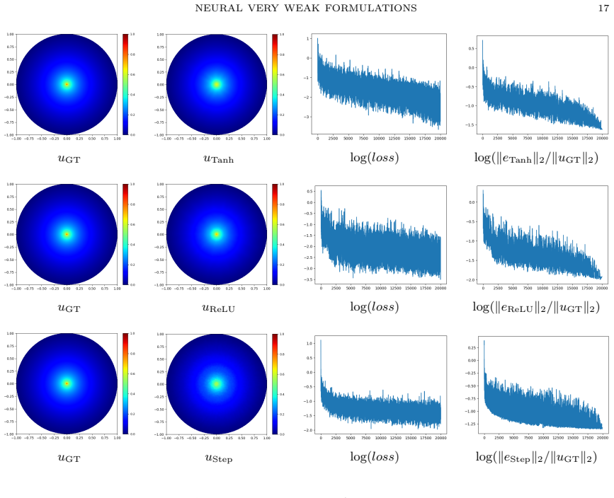
- 1-bit quantized (binary-weight) networks become a viable trial space for elliptic problems, with observed relative L2 errors of a few percent, opening the door to low-precision hardware inference.
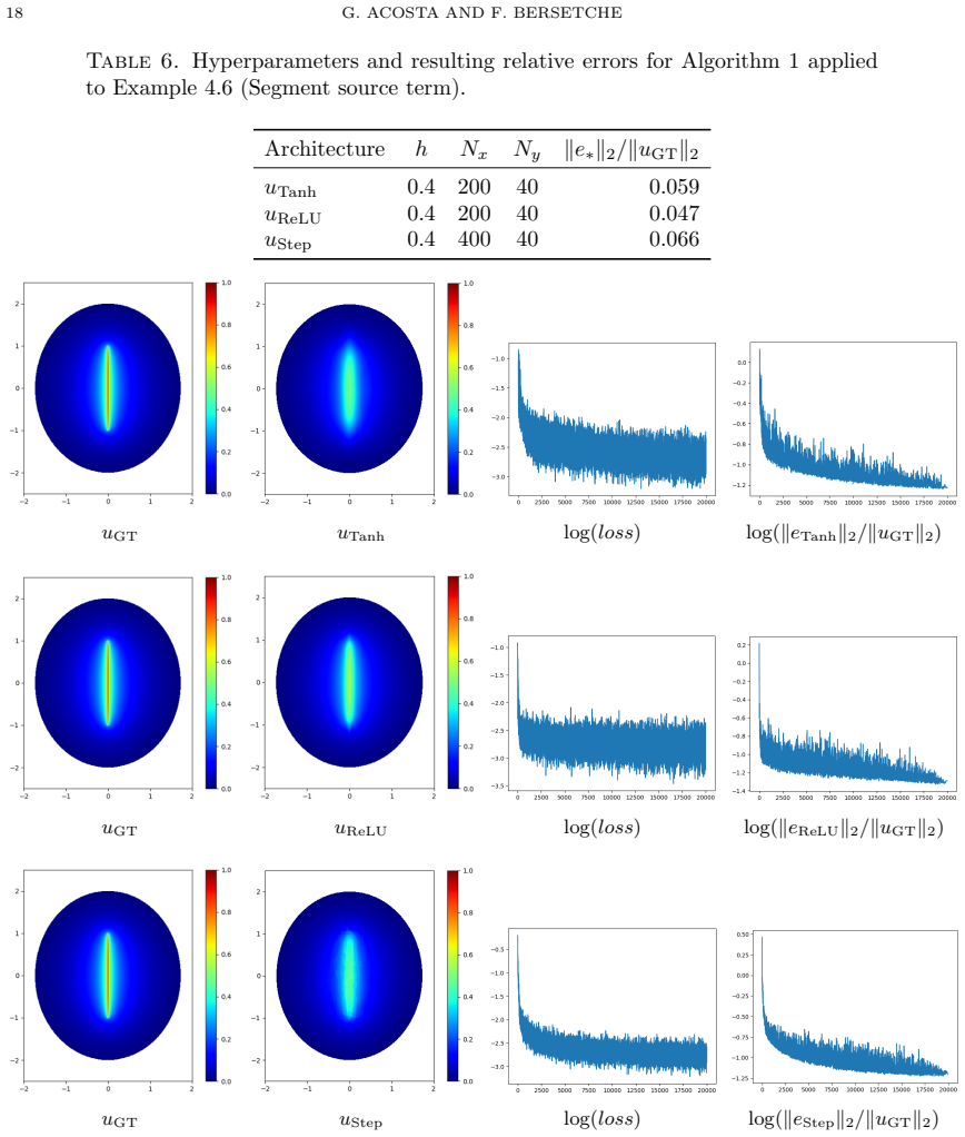
- Singular sources such as Dirac deltas and line-segment measures, as well as non-smooth domains, require no special regularization in this formulation.
- In the 20-dimensional test, the method attains about 1–2% relative L2 error, suggesting that very weak least-squares losses do not immediately hit the curse of dimensionality in that regime.
- The balanced sampling of Δrho_h effectively provides a centered difference operator, so the same machinery transfers to variable-coefficient second-order operators by sampling second partial derivatives.
Where Pith is reading between the lines
- A natural next test is to replace the smooth mollifier with kernels of higher order, extending the same 'no derivative of the trial' logic to higher-order and time-dependent PDEs; the paper only demonstrates elliptic second-order problems.
- Because the quadrature emulates a centered difference, the method might be stabilized by deterministic quasi-Monte Carlo or analytic integration of Δrho_h over simple network pieces, shrinking sample counts and reducing loss noise.
- The reported sensitivity to (h, N_x, N_y) suggests that an adaptive scheme tuning h and sample counts per iteration—or annealing h downward—could improve accuracy; the paper leaves this scaling open.
- If validated further, the formulation offers a path to neural solvers whose forward pass is almost entirely sign-and-accumulate operations, mapping directly onto binarized accelerators or field-programmable gate arrays.
Editorial analysis
A structured set of objections, weighed in public.
Referee Report
Summary. The paper proposes two least-squares very weak formulations (A1 and A2) for elliptic boundary value problems with homogeneous Dirichlet conditions. Trial functions are neural networks with low regularity; test functions are translations of a smooth compactly supported mollifier. The resulting losses are discretized by Monte Carlo with a balanced importance-sampling rule, avoiding automatic differentiation. The authors report relative L2 errors of roughly 0.2%–6.7% for Tanh, ReLU, step-activation, and 1-bit quantized step networks on problems in 1D, 2D, 3D, an L-shaped domain, and a 20D nonlinear example.
Significance. If made rigorous, the framework would be a useful proof of concept for hardware-oriented neural PDE solvers with binarized weights and step activations, and the avoidance of automatic differentiation is attractive. The paper contains explicit formulas for the mollifier Laplacian, an elementary density argument for quantized Heaviside networks, a broad set of numerical experiments, and an openly available implementation; these are strengths. However, the load-bearing A1 loss has a boundary-extension defect, the nonlinear example is not covered by the linear derivation, and there is no consistency or convergence analysis for the balanced quadrature. The central claim therefore is not yet established.
major comments (4)
- [§2.1, Eq. (2.4)] For centers x within h of ∂Ω, the ball B_h(x) in (2.4) exits Ω. Integrating by parts over the full ball and using the exact solution extended across the boundary yields an extra boundary-flux term ∫_{B_h∩∂Ω} ρ_h [∂u/∂η] dS, because the exterior extension is not part of the BVP and is not prescribed by f̃. This term is generically nonzero, so the true solution is not a zero of L; the minimizer depends on the arbitrary choice of f̃ outside Ω. The manuscript never specifies the extension or a compatibility condition. Algorithm 1 is used for Examples 4.1, 4.2, 4.4, 4.5 and 4.6, so those reported errors could reflect the extension artifact rather than the PDE residual. For f=δ and δ′, moreover, no smooth extension f̃ exists and Algorithm 1 is not defined as written.
- [Example 4.4] The problem solved is the nonlinear Sine-Gordon equation Δu + sin(u) = g, but the derivation in Section 2 and the losses (2.4)/(3.1) are for the linear equation −Δu = f. The paper does not state how the nonlinear term is incorporated. Replacing f(y) in (3.1) by g(y) − sin(uθ(y)) would make the 'source' depend on the trial function and would alter the Monte Carlo weights and the interpretation of C_f. No justification is given. This experiment is therefore not supported by the proposed formulation as written.
- [§2.1/§2.2, §3.5] The integration-by-parts identities are stated 'assuming a smooth enough uθ', but the trial functions are step/Heaviside discontinuous or ReLU and uθ = d0 vθ is only L2 or possibly discontinuous. A distributional interpretation of Δuθ is required to justify equating the bracketed term to zero; the manuscript provides none. Since the central claim is that low-regularity trial spaces are admissible, this is a load-bearing gap, not a cosmetic one.
- [§3.1, Eqs. (3.1)–(3.3)] The balanced Monte Carlo rule for ∫ u Δρ_h is heuristic and no error or bias analysis is provided. The sample counts N_y are small (20–200 in Tables 1–7) and h is relatively large, so the numerical minimizer may not be a faithful approximation of the continuous loss. No consistency or convergence of the empirical loss to the continuous functional is shown. Since the numerical results are the principal evidence for the paper's claim, at least a consistency argument or a numerical convergence study is needed.
minor comments (4)
- [Eq. (3.1) vs. Algorithm 1] Eq. (3.1) uses f(y), while Algorithm 1 Step 0 and §3.2 refer to a smooth extension f̃. If an extension is intended, the notation should be consistent and its construction specified; this ambiguity matters for the boundary issue in A1.
- [Table 7] In Example 4.7 there is no exact solution; the reference is u_FEM. The table header should read ∥e∗∥2/∥u_FEM∥2 instead of ∥e∗∥2/∥uGT∥2.
- [Example 4.4] The dimension d is not stated explicitly; the coefficient list has 19 entries, suggesting d=20. Please state d and verify that the sum index range matches the listed coefficients.
- [Example 4.3] There is a typo: 'For u Step integrates a neural network...' should be 'For u Step we integrate a neural network...'.
Circularity Check
No significant circularity: the numerical tests are manufactured-solution benchmarks, the loss functionals are derived from the PDE residual, and the only self-citation is contextual.
full rationale
The paper's central claim is that least-squares very weak formulations can be discretized with low-regularity neural networks. The losses (2.4)/(2.5) are built from the PDE residual (integrals of f + Δu_θ against smooth test functions), not from the target solution u_GT. In each example, f is manufactured from u_GT, but u_GT is then used only as an external benchmark for reporting relative L2 errors; no network parameter is fitted to u_GT. The only self-citation is [2] by co-author Bersetche, appearing in a literature-survey sentence about first-order system least squares methods; it does not support the VWF identity, the mollifier construction, the density result, or any numerical claim. Remark 3, which proves density of one-bit quantized Heaviside networks in L^p, is self-contained in the text via an explicit construction of parallelotope characteristic functions, following ideas from [20] but not relying on a self-citation. The concerns about the smooth extension f̃ in Algorithm 1 and about the Monte Carlo quadrature being faithful are correctness/well-posedness issues, not circular reductions: even if those concerns were valid, they would not make the derivation equivalent to its own inputs. The manuscript is self-contained against analytical or FEM reference solutions, so no load-bearing step reduces by construction to a fitted parameter or to a self-citation chain.
Axiom & Free-Parameter Ledger
free parameters (4)
- Mollifier support radius h =
0.15–0.4 depending on example/architecture
- Sampling counts N_x, N_f, N_y (and N_Γ for A2) =
e.g., N_x=20–400, N_y=20–200; N_f not individually tabulated
- Network architecture sizes and augmented linear units s =
N(4,(64,64),6) up to N(4,(2048,2048),4), plus 128-neuron two-layer baselines
- Optimizer and learning-rate schedule =
Adam, initial LR 1e-3–1e-2, linear decay to zero
axioms (6)
- standard math The continuous VWF (2.2) is well-posed via classical inf-sup arguments.
- standard math Translation-invariant spaces generated by ρ_h are sufficiently rich to approximate functions up to a small saturation error.
- domain assumption A smooth signed-distance surrogate d^S exists near ∂Ω for smooth domains, and a distance surrogate with ∂d/∂η = 1 a.e. exists for the non-smooth domains used.
- domain assumption Sobolev extension of f (and u) across ∂Ω preserves enough smoothness for the fictitious-domain-style loss.
- ad hoc to paper The balanced importance-sampling Monte Carlo rule for ∫ u Δρ_h is an adequate approximation and emulates a centered difference operator.
- ad hoc to paper Integrals over B_h(x)∩Ω and B_h(x)∩∂Ω may be replaced by integrals over B_h(x) and ∂Ω with zero extensions.
read the original abstract
We show, as a proof of concept, that least-squares very weak formulations of elliptic problems can be effectively discretized by neural networks possessing low regularity, provided the test functions are drawn from appropriately smooth spaces. Apart from the immediate computational benefit of avoiding automatic differentiation, this approach, evaluated across various neural network spaces, demonstrates good performance even in challenging contexts, such as singular solutions and high dimensional settings. Particular attention is paid to trial functions based on step activations and one bit quantized linear functions, which are amenable to efficient hardware-oriented implementations.
Figures



Reference graph
Works this paper leans on
-
[1]
A. A. Balinsky, W. D. Evans, and R. T. Lewis.Hardy’s Inequality on Domains, pages 77–134. Springer Inter- national Publishing, Cham, 2015
2015
-
[2]
Bersetche and J
F. Bersetche and J. P. Borthagaray. A deep first-order system least squares method for solving elliptic PDEs. Comput. Math. Appl., 129:136–150, 2023
2023
-
[3]
M. Courbariaux, I. Hubara, D. Soudry, R. El-Yaniv, and Y. Bengio. Binarized neural networks: Training deep neural networks with weights and activations constrained to+ 1 or-1.arXiv preprint arXiv:1602.02830, 2016
Pith/arXiv arXiv 2016
-
[4]
W. E and S. Wojtowytsch. Some observations on high-dimensional partial differential equations with Barron data. InProc. Math. Sci. Mach. Learn., pages 253–269, 2022
2022
-
[5]
W. E and B. Yu. The deep Ritz method: A deep learning-based numerical algorithm for solving variational problems.Commun. Math. Stat., 6(1):1–12, 2018
2018
-
[6]
L. C. Evans.Partial differential equations, volume 19 ofGrad. Stud. Math.Providence, RI: American Mathe- matical Society (AMS), 2nd ed. edition, 2010
2010
-
[7]
Glowinski, T.-W
R. Glowinski, T.-W. Pan, and J. Periaux. Fictitious domain method for the Dirichlet problem and its general- ization to some flow problems. InFinite elements in fluids: new trends and applications. Proceedings of the 8th NEURAL VERY WEAK FORMULATIONS 21 international conference, Barcelona, Spain, September 20-23, 1993. Part I, pages 347–368. Barcelona: Ce...
1993
-
[8]
Grisvard.Elliptic problems in nonsmooth domains, volume 24 ofMonogr
P. Grisvard.Elliptic problems in nonsmooth domains, volume 24 ofMonogr. Stud. Math.Pitman, Boston, MA, 1985
1985
-
[9]
C. He, X. Hu, and L. Mu. A mesh-free method using piecewise deep neural network for elliptic interface problems. J. Comput. Appl. Math., 412:114358, 2022
2022
-
[10]
Z. Hu, Z. Shi, G. E. Karniadakis, and K. Kawaguchi. Hutchinson trace estimation for high-dimensional and high- order physics-informed neural networks.Computer Methods in Applied Mechanics and Engineering, 424:116883, 2024
2024
-
[11]
Z. Hu, K. Shukla, G. E. Karniadakis, and K. Kawaguchi. Tackling the curse of dimensionality with physics- informed neural networks.Neural Networks, 176:106369, 2024
2024
-
[12]
Z. Hu, Z. Yang, Y. Wang, G. E. Karniadakis, and K. Kawaguchi. Bias-variance trade-off in physics-informed neural networks with randomized smoothing for high-dimensional pdes.SIAM Journal on Scientific Computing, 47(4):C846–C872, 2025
2025
-
[13]
I. Kong, J. Chen, S. Langer, and J. Schmidt-Hieber. On the expressivity of deep heaviside networks.arXiv preprint arXiv:2505.00110, 2025
Pith/arXiv arXiv 2025
-
[14]
J. L. Lions and E. Magenes.Non-homogeneous boundary value problems and applications. Vol. I,II,III. Trans- lated from the French by P. Kenneth. Grundlehren Math. Wiss. Springer, Cham, 1972
1972
-
[15]
Liu and Z
M. Liu and Z. Cai. Adaptive two-layer ReLU neural network: Ii. Ritz approximation to elliptic PDEs.Comput. Math. Appl., 113:103–116, 2022
2022
-
[16]
M. Liu, Z. Cai, and J. Chen. Adaptive two-layer ReLU neural network: I. best least-squares approximation. Comput. Math. Appl., 113:34–44, 2022
2022
-
[17]
Maz’ya and G
V. Maz’ya and G. Schmidt.Approximate approximations, volume 141 ofMath. Surv. Monogr.Providence, RI: American Mathematical Society (AMS), 2007
2007
-
[18]
Nikolov and P
N. Nikolov and P. J. Thomas. Boundary regularity for the distance functions, and the eikonal equation.J. Geom. Anal., 35(8):8, 2025. Id/No 230
2025
-
[19]
J. A. A. Opschoor, P. C. Petersen, and C. Schwab. First order system least squares neural networks.arXiv preprint, arXiv:2409.20264, 2024
Pith/arXiv arXiv 2024
-
[20]
A. Pinkus. Approximation theory of the MLP model in neural networks. InActa Numerica, volume 8, pages 143–195. Cambridge University Press, 1999
1999
-
[21]
Raissi, P
M. Raissi, P. Perdikaris, and G. E. Karniadakis. Physics-informed neural networks: A deep learning framework for solving forward and inverse problems involving nonlinear partial differential equations.J. Comput. Phys., 378:686–707, 2019
2019
-
[22]
Sirignano and K
J. Sirignano and K. Spiliopoulos. Dgm: A deep learning algorithm for solving partial differential equations.J. Comput. Phys., 375:1339–1364, 2018
2018
-
[23]
Umuroglu, N
Y. Umuroglu, N. J. Fraser, G. Gambardella, M. Blott, P. Leong, M. Jahre, and K. Vissers. Finn: A framework for fast, scalable binarized neural network inference. InProceedings of the 2017 ACM/SIGDA international symposium on field-programmable gate arrays, pages 65–74, 2017
2017
-
[24]
Wojtowytsch and W
S. Wojtowytsch and W. E. Can shallow neural networks beat the curse of dimensionality? a mean field training perspective.IEEE Trans. Artif. Intell., 1(2):121–129, 2020
2020
-
[25]
J. Xu. Finite neuron method and convergence analysis.Commun. Comput. Phys., 28:1707–1745, 2020. (G. Acosta)Departamento de Matem ´atica, FCEyN, Universidad de Buenos Aires / IMAS, CONICET, Buenos Aires, Argentina Email address:gacosta@dm.uba.ar (F. Bersetche)Departamento de Matem ´atica, FCEyN, Universidad de Buenos Aires / IMAS, CONICET, Buenos Aires, Ar...
2020
discussion (0)
Sign in with ORCID, Apple, or X to comment. Anyone can read and Pith papers without signing in.