REVIEW 3 major objections 4 minor 76 references
This paper argues that split complex-valued physics-informed neural networks solve forward and inverse nonlinear PDEs more accurately than real-valued ones.
Reviewed by Pith at T0; open to challenge. T0 means a machine referee read the full paper against a public rubric. the ladder, T0–T4 →
Split complex-valued PINNs achieve lower benchmark errors than real-valued PINNs, but the comparison is confounded by doubled parameters and unresolved internal error inconsistencies.
T0 review reviewed 2026-08-02 challenge →
load-bearing objection Broad benchmark suite for split-complex PINNs, but the headline claim is not yet supported: the comparison against real PINNs is confounded by parameter count, and the reported Burgers error does not reproduce in the ablation tables. the 3 major comments →
Split Complex-Valued Physics-Informed Neural Networks for Forward and Inverse Nonlinear PDEs
The pith
A machine-rendered reading of the paper's core claim, the machinery that carries it, and where it could break.
The reading
Core claim
The central claim is that moving the trainable weights, biases, and latent features of a PINN into the complex domain — while keeping activations split (real functions applied to real and imaginary parts independently) — yields a strictly more expressive approximator that still trains with standard real-valued optimizers. The network output's real part is the physical solution; the imaginary part is a free auxiliary field that enriches the approximation without altering the physics loss. The authors show that this construction matches or beats conventional real-valued PINNs across a wide suite of nonlinear, oscillatory, and high-dimensional problems, with the 3D Beltrami flow reaching a rela
What carries the argument
The core object is the split complex-valued multilayer perceptron: weights and biases are complex, inputs are embedded as complex numbers with zero imaginary part, and the activation function is applied independently to the real and imaginary components (e.g., split GELU or split tanh). This preserves the amplitude–phase coupling of complex multiplication while avoiding holomorphic activation restrictions imposed by Liouville's theorem. The physical prediction is the real part of the output, so the imaginary part acts as an auxiliary latent channel. Training uses a split view: the optimizer operates on real and imaginary parts as real variables, with Adam followed by L-BFGS.
Load-bearing premise
The load-bearing premise is that the accuracy gains come from the complex-valued architecture itself, rather than from the roughly doubled number of trainable parameters or from the discarded imaginary part of the output acting as an unpenalized auxiliary variable.
What would settle it
Run a matched-parameter-count comparison: for each SCV-PINN, construct a real-valued MLP with the same number of real trainable parameters (e.g., double the hidden width) and train it with the same Adam/L-BFGS budget on the same collocation points. If that real network matches or beats SCV-PINN's relative L2 errors, the central claim is a parameter-count effect, not a complex-structure effect. A second check: freeze the imaginary part of the output to zero after initialization (so only real-part weights train) and see whether accuracy collapses; if it does not, the imaginary channel is not doi
If this is right
- If the reported accuracy holds, SCV-PINNs can be dropped into existing PINN pipelines as a direct replacement for real-valued networks without changing the loss formulation or optimizer.
- The method extends naturally to intrinsically complex-valued equations such as nonlinear Schrödinger, where both real and imaginary parts of the solution are recovered simultaneously from the complex output.
- Improved parameter identification for inverse Burgers and Navier–Stokes problems suggests the framework could be applied to data-driven discovery of unknown physical coefficients in experiments.
- The high accuracy on the 3D Beltrami flow benchmark indicates that complex-valued representations may help with high-dimensional, smoothly oscillatory Navier–Stokes solutions.
Where Pith is reading between the lines
- The imaginary channel is never used in the final prediction, so SCV-PINN could be seen as an adaptive augmentation of the function space; a natural test is whether a real-valued network with an explicit auxiliary output channel (not used in the loss) matches the gains.
- Because the paper's ablation shows ReLU-type split activations stall under L-BFGS, future variants for second-order optimizers should stick to smooth activations; this may also explain why some complex-valued PINN efforts reported unstable training.
- If the benefit is genuinely from complex multiplication's phase coupling, the approach could be combined with Fourier-feature embeddings to push further into the high-frequency regime, though this is a speculation beyond the present results.
- The authors do not report wall-clock times or parameter counts per benchmark; a practical reader would want to know the computational cost per unit accuracy before adopting the method.
Editorial analysis
A structured set of objections, weighed in public.
Referee Report
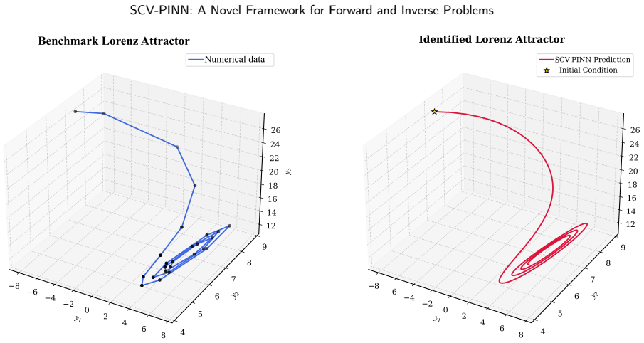
Summary. The paper proposes split complex-valued physics-informed neural networks (SCV-PINNs), in which weights, biases, and latent representations are complex-valued while activation functions are applied separately to the real and imaginary parts. The physical solution is recovered as the real part of the network output. The method is evaluated on a wide range of forward and inverse benchmarks: Burgers, Allen–Cahn, KdV, nonlinear Schrödinger, Helmholtz on regular/irregular domains, Poisson on regular/L-shaped domains, Kovasznay flow, lid-driven cavity flow, Lorenz system identification, inverse Burgers, inverse Navier–Stokes, and a 3D Beltrami flow. The central claim is that SCV-PINNs consistently achieve significantly lower relative L2 errors and better parameter identification than real-valued PINNs and existing variants. Extensive ablations of split activation functions and sampling strategies are also reported.
Significance. If the central claim is correct, SCV-PINN would be a broadly applicable and practically useful extension of standard PINNs, particularly for oscillatory and phase-dependent problems. The manuscript's strengths are the breadth of benchmarks, the systematic ablation of activations and collocation sampling, and the clear presentation of the method. However, the load-bearing comparison is currently confounded by a parameter-count effect, and several internal inconsistencies in the reported numerical values prevent the claims from being verified as stated. The paper does not provide code or any measure of run-to-run variability, which further limits reproducibility. With additional control experiments and correction of the inconsistencies, the contribution could become solid; in its present form the evidence for the central claim is not yet sufficient.
major comments (3)
- [Sec. 4.3, Eqs. (58)–(62); Sec. 4.4.3, Eqs. (72)–(73); Sec. 4.4.1, Eq. (67); Table 10] The 'identical architecture' comparisons in Table 10 are not parameter-matched. A complex hidden layer with m units stores 2m real-valued parameters, so an m-unit complex SCV-PINN has roughly twice as many trainable parameters as an m-unit real RV-PINN. Since the physical output is taken as the real part (Eq. 67), the imaginary branch is an auxiliary latent representation that approximately doubles representational capacity. No real-valued baseline with doubled width (2m units) and otherwise identical settings is reported anywhere. The central claim—that the improvement is due to the split-complex structure rather than to parameter count—is therefore not yet supported. A same-parameter-count real MLP control is essential.
- [Sec. 5.4; Table 1; Table 9; Table 10; Appendix B, Table 12] The Burgers forward problem is reported with a relative L2 error of 6.73e-5 in Table 1/Table 9 and Sec. 5.4, but Table 10 (under 'identical hyperparameters') lists a relative L2 error of 1.09e-2 for the same problem. Appendix B, Table 12, reports 1.244e-2 for LHS with CGELU and 1.090e-2 for random sampling, which matches the Table 10 value but not the headline 6.73e-5. The paper does not explain which configuration produces the headline error, and which configuration is used in the fair comparison. This is a direct, quantifiable inconsistency in the central numerical evidence and must be resolved.
- [Sec. 5.13, Eq. (170); Table 7; Fig. 24 caption] The 'true' parameters for the inverse Navier–Stokes problem are inconsistent. The text (Eq. 170) states the exact values are λ1=1.0, λ2=0.01. Table 7 reports the true values as 1.00137 and 0.01000, while Fig. 24's caption states the exact values are 1.00137 and 0.01007. Without a single consistent reference, the reported parameter-identification accuracy cannot be evaluated, and the comparison against the vanilla-PINN is ambiguous.
minor comments (4)
- [Sec. 5.1, Eq. (102); Sec. 5.5, Eq. (117)] Typos: '2,sech(x)' should read '2 sech(x)', and '0.0001, u_xx' should read '0.0001 u_xx'.
- [Tables 9 and 10] The same benchmark problems appear with different relative L2 errors in Table 9 and Table 10 (e.g., Kovasznay u: 8.20e-5 vs 1.22e-4; Helmholtz regular: 2.17e-4 vs 6.14e-3). The paper should clarify that these correspond to different training budgets or configurations, and should state which table supports the headline claims.
- [Appendices A and B] The selection of CTanh/CGELU and LHS as the default choices is based on ablations performed on the Burgers benchmark, which is also a headline problem. This is a form of selection bias on the evaluation benchmarks; the authors should acknowledge this and, ideally, validate on a separate tuning set.
- [Data Availability] The statement says data are available upon request but no code is provided. For a scientific machine learning paper, releasing training code at least for the main experiments would substantially improve reproducibility. Additionally, all results appear to be single-run; reporting mean±std over multiple seeds would strengthen the claim of 'consistent' improvement.
Circularity Check
No circular derivation found: the paper is an empirical architecture study with external benchmarks; the main comparisons are experimental, not definitionally forced.
full rationale
The paper's central claims are numerical: SCV-PINN achieves lower relative L2 errors on standard forward and inverse PDE benchmarks (Burgers, Allen–Cahn, NLS, Helmholtz, Kovasznay, cavity, Lorenz, inverse Navier–Stokes, 3D Beltrami flow). These are measured against closed-form or reference solutions, not derived from the method's definition. The physical output is taken as the real part of the complex network output (Eqs. 67 and 94), but this is a stated modeling choice rather than a hidden reuse of the target result. The comparisons with RV-PINN in Table 10 are genuine experiments, although the 'identical architecture' protocol leaves the complex network with roughly twice the real parameter count; that is a possible experimental confound and a correctness/interpretability concern, but it is not a circular reduction: the improved errors are not forced by construction, and the paper does not define SCV-PINN's advantage in terms of the benchmarks it then reports. The two self-citations ([61], [62]) are contextual related-work mentions and are not load-bearing for the main claim. The ablation-based choices of activation functions and sampling strategies (Appendices A/B) are hyperparameter selections made before the headline results, not fitted values disguised as predictions. No step in the paper equates a prediction with an input by definition, so the circularity score is 0.
Axiom & Free-Parameter Ledger
free parameters (4)
- Per-benchmark network architecture =
e.g., Burgers 8x20 CTanh; NLS 5x100 CGELU; 3D Beltrami 2x40 CGELU
- Per-benchmark training schedule =
5,000/5,000 to 10,000/20,000 Adam/L-BFGS iterations
- Collocation point count and sampling strategy =
e.g., 10,000 LHS (Burgers); 20,000 LHS (NLS/Allen-Cahn); 2,000 (Helmholtz hole)
- Loss weights λ_f, λ_u, λ_d =
not reported
axioms (3)
- ad hoc to paper A real-valued MLP with the same layer width is a fair control for SCV-PINN.
- domain assumption The imaginary component enriches the approximation space without affecting the physical output.
- domain assumption A single run per configuration is representative.
invented entities (1)
-
Auxiliary imaginary latent representation
no independent evidence
Cite this review
Pith. "Pith review of Split Complex-Valued Physics-Informed Neural Networks for Forward and Inverse Nonlinear PDEs." pith.science (2026). https://pith.science/paper/UIZYF7AF
@misc{pith2026260715087,
  author       = {Pith},
  title        = {Pith review of: Split Complex-Valued Physics-Informed Neural Networks for Forward and Inverse Nonlinear PDEs},
  year         = {2026},
  howpublished = {\url{https://pith.science/paper/UIZYF7AF}},
  note         = {Machine review of arXiv:2607.15087}
}
read the original abstract
Physics-informed neural networks (PINNs) have emerged as a powerful framework for solving forward and inverse partial differential equations (PDEs), but conventional real-valued PINNs (RV-PINNs) often suffer from spectral bias, limited expressivity, and reduced accuracy for high-frequency, oscillatory, and phase-dependent dynamics. In this work, we propose a generalized split complex-valued physics-informed neural network (SCV-PINN), in which network parameters and latent representations are defined in the complex domain. The framework employs split complex-valued activation functions by independently applying standard real-valued activations to the real and imaginary components, providing numerical stability, computational efficiency, and improved approximation capability. This formulation enables simultaneous learning of amplitude and phase information, enhancing the representation of nonlinear and oscillatory systems. Extensive ablation studies evaluate different split activation functions and collocation sampling strategies. The proposed framework is validated on forward and inverse PDE benchmarks including Burgers, Allen-Cahn, Korteweg-de Vries, nonlinear Schrodinger, Helmholtz, Poisson, Kovasznay flow (Re = 20), lid-driven cavity flow (Re = 100), the Lorenz system, inverse Burgers, inverse Navier-Stokes (Re = 100), and a three-dimensional Navier-Stokes Beltrami flow. For the Beltrami benchmark, SCV-PINN achieves a relative L2 error of 4.07 x 10^-5. Numerical results consistently demonstrate lower relative L2 errors and more accurate parameter identification than RV-PINNs and several existing PINN variants. The proposed SCV-PINN provides a robust and generalized extension of standard PINNs for complex-valued, multiscale, oscillatory, high-dimensional, and real-valued nonlinear PDEs.
Figures




Reference graph
Works this paper leans on
-
[1]
and Bengio, Y., 2016
Goodfellow, I., Bengio, Y., Courville, A. and Bengio, Y., 2016. Deep learning (Vol. 1, No. 2, pp. 1-800). Cambridge: MIT press
2016
-
[2]
and Nasrabadi, N.M., 2006
Bishop, C.M. and Nasrabadi, N.M., 2006. Pattern recognition and machine learning (Vol. 4, No. 4, p. 738). New York: springer
2006
-
[3]
and Bishop, H., 2023
Bishop, C.M. and Bishop, H., 2023. Deep learning: Foundations and concepts. Springer Nature
2023
-
[4]
Neural networks and deep learning (Vol
Aggarwal, C.C., 2018. Neural networks and deep learning (Vol. 10, No. 978, p. 3). Cham: Springer
2018
-
[5]
Linear algebra and learning from data (Vol
Strang, G., 2019. Linear algebra and learning from data (Vol. 4). Cambridge: Wellesley-Cambridge Press
2019
-
[6]
Zhang, C., Bengio, S., Hardt, M., Recht, B. and Vinyals, O., 2016. Understanding deep learning requires rethinking generalization. arXiv preprint arXiv:1611.03530
Pith/arXiv arXiv 2016
-
[7]
and Kress, R., 1999
Krantz, S.G., Kress, S. and Kress, R., 1999. Handbook of complex variables (p. 290). Boston: Birkhäuser
1999
-
[8]
and Silverman, H., 2006
Ponnusamy, S. and Silverman, H., 2006. Complex variables with applications. Boston, MA: Birkhäuser Boston
2006
-
[9]
and Shanahan, P., 2009
Zill, D. and Shanahan, P., 2009. A first course in complex analysis with applications. Jones & Bartlett Learning
2009
-
[10]
and Savitha, R., 2013
Suresh, S., Sundararajan, N. and Savitha, R., 2013. Supervised learning with complex-valued neural networks (Vol. 48). Berlin: Springer
2013
-
[11]
On complex valued convolutional neural networks
Guberman, N., 2016. On complex valued convolutional neural networks. arXiv preprint arXiv:1602.09046
Pith/arXiv arXiv 2016
-
[12]
arXiv preprint arXiv:2302.08286
Barrachina,J.A.,Ren,C.,Vieillard,G.,Morisseau,C.andOvarlez,J.P.,2023.Theoryandimplementationofcomplex-valuedneuralnetworks. arXiv preprint arXiv:2302.08286
Pith/arXiv arXiv 2023
-
[13]
Complex-valued Neural Networks–Theory and Analysis
Abdalla, R., 2023. Complex-valued Neural Networks–Theory and Analysis. arXiv preprint arXiv:2312.06087
Pith/arXiv arXiv 2023
-
[14]
and Gao, S., 2022
Lee, C., Hasegawa, H. and Gao, S., 2022. Complex-valued neural networks: A comprehensive survey. IEEE/CAA Journal of Automatica Sinica, 9(8), pp.1406-1426
2022
-
[15]
Bassey, J., Qian, L. and Li, X., 2021. A survey of complex-valued neural networks. arXiv preprint arXiv:2101.12249
Pith/arXiv arXiv 2021
-
[16]
and Pernkopf, F., 2021, May
Fuchs, A., Rock, J., Toth, M., Meissner, P. and Pernkopf, F., 2021, May. Complex-valued convolutional neural networks for enhanced radar signal denoising and interference mitigation. In 2021 IEEE Radar Conference (RadarConf21) (pp. 1-6). IEEE
2021
-
[17]
Scarnati,T.andLewis,B.,2021,May.Complex-valuedneuralnetworksforsyntheticapertureradarimageclassification.In2021IEEERadar Conference (RadarConf21) (pp. 1-6). IEEE
2021
-
[18]
and Lee, K., 2018, September
Choi, H.S., Kim, J.H., Huh, J., Kim, A., Ha, J.W. and Lee, K., 2018, September. Phase-aware speech enhancement with deep complex u-net. In International Conference on Learning Representations
2018
-
[19]
and Weidmann, U., 2014
Fink, O., Zio, E. and Weidmann, U., 2014. Predicting component reliability and level of degradation with complex-valued neural networks. Reliability Engineering & System Safety, 121, pp.198-206
2014
-
[20]
Trabelsi, C., Bilaniuk, O., Zhang, Y., Serdyuk, D., Subramanian, S., Santos, J.F., Mehri, S., Rostamzadeh, N., Bengio, Y. and Pal, C.J., 2017. Deep complex networks. arXiv preprint arXiv:1705.09792
Pith/arXiv arXiv 2017
-
[21]
Complex-valued neural networks
Hirose, A., 2006. Complex-valued neural networks. Berlin, Heidelberg: Springer Berlin Heidelberg
2006
-
[22]
Reichert, D.P. and Serre, T., 2013. Neuronal synchrony in complex-valued deep networks. arXiv preprint arXiv:1312.6115
Pith/arXiv arXiv 2013
-
[23]
Solving the XOR problem and the detection of symmetry using a single complex-valued neuron
Nitta, T., 2003. Solving the XOR problem and the detection of symmetry using a single complex-valued neuron. Neural Networks, 16(8), pp.1101-1105
2003
-
[24]
On the inherent property of the decision boundary in complex-valued neural networks
Nitta, T., 2003. On the inherent property of the decision boundary in complex-valued neural networks. Neurocomputing, 50, pp.291-303
2003
-
[25]
An analysis of the fundamental structure of complex-valued neurons
Nitta, T., 2000. An analysis of the fundamental structure of complex-valued neurons. Neural Processing Letters, 12(3), pp.239-246
2000
-
[26]
Complex-valued neural networks: Advances and applications [book review]
Tanaka, G., 2013. Complex-valued neural networks: Advances and applications [book review]. ieee Computational intelligenCe magazine, 8(2), pp.77-79
2013
-
[27]
Appendix a: Wirtinger calculus
Fischer, R.F., 2002. Appendix a: Wirtinger calculus
2002
-
[28]
Zur formalen theorie der funktionen von mehr komplexen veränderlichen
Wirtinger, W., 1927. Zur formalen theorie der funktionen von mehr komplexen veränderlichen. Mathematische Annalen, 97(1), pp.357-375
1927
-
[29]
and Hirose, A., 2013
Amin, M.F., Murase, K. and Hirose, A., 2013. Learning algorithms in complex-valued neural networks using Wirtinger calculus. Complex- Valued Neural Networks: Advances and Applications, pp.75-102
2013
-
[30]
and Murase, K., 2011, November
Amin, M.F., Amin, M.I., Al-Nuaimi, A.Y.H. and Murase, K., 2011, November. Wirtinger calculus based gradient descent and Levenberg- Marquardt learning algorithms in complex-valued neural networks. In International Conference on Neural Information Processing (pp. 550- 559). Berlin, Heidelberg: Springer Berlin Heidelberg
2011
-
[31]
Hammad, M.M., 2024. Comprehensive survey of complex-valued neural networks: Insights into backpropagation and activation functions. arXiv preprint arXiv:2407.19258. Barman, Ray, Chatterjee:Preprint submitted to ElsevierPage 52 of 54 SCV-PINN: A Novel Framework for Forward and Inverse Problems
Pith/arXiv arXiv 2024
-
[32]
Journal of Computational physics, 378, pp.686-707
Raissi,M.,Perdikaris,P.andKarniadakis,G.E.,2019.Physics-informedneuralnetworks:Adeeplearningframeworkforsolvingforwardand inverse problems involving nonlinear partial differential equations. Journal of Computational physics, 378, pp.686-707
2019
-
[33]
and Yang, L., 2021
Karniadakis, G.E., Kevrekidis, I.G., Lu, L., Perdikaris, P., Wang, S. and Yang, L., 2021. Physics-informed machine learning. Nature Reviews Physics, 3(6), pp.422-440
2021
-
[34]
and Piccialli, F., 2022
Cuomo, S., Di Cola, V.S., Giampaolo, F., Rozza, G., Raissi, M. and Piccialli, F., 2022. Scientific machine learning through physics–informed neural networks: Where we are and what’s next. Journal of Scientific Computing, 92(3), p.88
2022
-
[35]
and Karniadakis, G.E., 2020
Raissi, M., Yazdani, A. and Karniadakis, G.E., 2020. Hidden fluid mechanics: Learning velocity and pressure fields from flow visualizations. Science, 367(6481), pp.1026-1030
2020
-
[36]
and Wang, J.X., 2020
Sun, L., Gao, H., Pan, S. and Wang, J.X., 2020. Surrogate modeling for fluid flows based on physics-constrained deep learning without simulation data. Computer Methods in Applied Mechanics and Engineering, 361, p.112732
2020
-
[37]
Raissi,M.,Wang,Z.,Triantafyllou,M.S.andKarniadakis,G.E.,2019.Deeplearningofvortex-inducedvibrations.Journaloffluidmechanics, 861, pp.119-137
2019
-
[38]
and Karniadakis, G.E., 2021
Jin, X., Cai, S., Li, H. and Karniadakis, G.E., 2021. NSFnets (Navier-Stokes flow nets): Physics-informed neural networks for the incompressible Navier-Stokes equations. Journal of Computational Physics, 426, p.109951
2021
-
[39]
and Perdikaris, P., 2020
Kissas, G., Yang, Y., Hwuang, E., Witschey, W.R., Detre, J.A. and Perdikaris, P., 2020. Machine learning in cardiovascular flows modeling: Predictingarterialbloodpressurefromnon-invasive4DflowMRIdatausingphysics-informedneuralnetworks.Computermethodsinapplied mechanics and engineering, 358, p.112623
2020
-
[40]
Liu,D.andWang,Y.,2019.Multi-fidelityphysics-constrainedneuralnetworkanditsapplicationinmaterialsmodeling.JournalofMechanical Design, 141(12), p.121403
2019
-
[41]
and Perdikaris, P., 2019
Yang, Y. and Perdikaris, P., 2019. Adversarial uncertainty quantification in physics-informed neural networks. Journal of Computational Physics, 394, pp.136-152
2019
-
[42]
Journal of computational physics, 394, pp.56-81
Zhu,Y.,Zabaras,N.,Koutsourelakis,P.S.andPerdikaris,P.,2019.Physics-constraineddeeplearningforhigh-dimensionalsurrogatemodeling and uncertainty quantification without labeled data. Journal of computational physics, 394, pp.56-81
2019
-
[43]
Journal of Computational Physics, 425, p.109913
Yang,L.,Meng,X.andKarniadakis,G.E.,2021.B-PINNs:Bayesianphysics-informedneuralnetworksforforwardandinversePDEproblems with noisy data. Journal of Computational Physics, 425, p.109913
2021
-
[44]
andE,W., 2018.Solving high-dimensionalpartialdifferential equationsusing deeplearning.Proceedings oftheNational Academy of Sciences, 115(34), pp.8505-8510
Han,J., Jentzen,A. andE,W., 2018.Solving high-dimensionalpartialdifferential equationsusing deeplearning.Proceedings oftheNational Academy of Sciences, 115(34), pp.8505-8510
2018
-
[45]
Pang,G.,Lu,L.andKarniadakis,G.E.,2019.fPINNs:Fractionalphysics-informedneuralnetworks.SIAMJournalonScientificComputing, 41(4), pp.A2603-A2626
2019
-
[46]
and Tchelepi, H.A., 2020
Fuks, O. and Tchelepi, H.A., 2020. Limitations of physics informed machine learning for nonlinear two-phase transport in porous media. Journal of Machine Learning for Modeling and Computing, 1(1)
2020
-
[47]
and Mahoney, M.W., 2021
Krishnapriyan, A., Gholami, A., Zhe, S., Kirby, R. and Mahoney, M.W., 2021. Characterizing possible failure modes in physics-informed neural networks. Advances in neural information processing systems, 34, pp.26548-26560
2021
-
[48]
and Perdikaris, P., 2021
Wang, S., Teng, Y. and Perdikaris, P., 2021. Understanding and mitigating gradient flow pathologies in physics-informed neural networks. SIAM Journal on Scientific Computing, 43(5), pp.A3055-A3081
2021
-
[49]
and Perdikaris, P., 2022
Wang, S., Yu, X. and Perdikaris, P., 2022. When and why PINNs fail to train: A neural tangent kernel perspective. Journal of Computational Physics, 449, p.110768
2022
-
[50]
and Courville, A., 2019, May
Rahaman, N., Baratin, A., Arpit, D., Draxler, F., Lin, M., Hamprecht, F., Bengio, Y. and Courville, A., 2019, May. On the spectral bias of neural networks. In International conference on machine learning (pp. 5301-5310). PMLR
2019
-
[51]
Cao, Y., Fang, Z., Wu, Y., Zhou, D.X. and Gu, Q., 2019. Towards understanding the spectral bias of deep learning. arXiv preprint arXiv:1912.01198
Pith/arXiv arXiv 2019
-
[52]
and Ng, R., 2020
Tancik, M., Srinivasan, P., Mildenhall, B., Fridovich-Keil, S., Raghavan, N., Singhal, U., Ramamoorthi, R., Barron, J. and Ng, R., 2020. Fourierfeaturesletnetworkslearnhighfrequencyfunctionsinlowdimensionaldomains.Advancesinneuralinformationprocessingsystems, 33, pp.7537-7547
2020
-
[53]
and Kritchman, S., 2020, November
Basri, R., Galun, M., Geifman, A., Jacobs, D., Kasten, Y. and Kritchman, S., 2020, November. Frequency bias in neural networks for input of non-uniform density. In International conference on machine learning (pp. 685-694). PMLR
2020
-
[54]
and Hongler, C., 2018
Jacot, A., Gabriel, F. and Hongler, C., 2018. Neural tangent kernel: Convergence and generalization in neural networks. Advances in neural information processing systems, 31
2018
-
[55]
and Braga-Neto, U.M., 2023
McClenny, L.D. and Braga-Neto, U.M., 2023. Self-adaptive physics-informed neural networks. Journal of Computational Physics, 474, p.111722
2023
-
[56]
Song,Y.,Wang,H.,Yang,H.,Taccari,M.L.andChen,X.,2024.Loss-attentionalphysics-informedneuralnetworks.JournalofComputational Physics, 501, p.112781
2024
-
[57]
and Ghosh, S., 2022
Mattey, R. and Ghosh, S., 2022. A novel sequential method to train physics informed neural networks for Allen Cahn and Cahn Hilliard equations. Computer Methods in Applied Mechanics and Engineering, 390, p.114474
2022
-
[58]
Journal of Fluids and Structures, 139, p.104421
Sundar,R.,Lucor,D.andSarkar,S.,2025.SequentiallearningbasedPINNstoovercometemporaldomaincomplexitiesinunsteadyflowpast flapping wings. Journal of Fluids and Structures, 139, p.104421
2025
-
[59]
Zhao,Z.,Ding,X.andPrakash,B.A.,2023.Pinnsformer:Atransformer-basedframeworkforphysics-informedneuralnetworks.arXivpreprint arXiv:2307.11833
Pith/arXiv arXiv 2023
-
[60]
and Liu, L., 2026
Zhu, Z., Huang, Y. and Liu, L., 2026. Physicssolver: Transformer-enhanced physics-informed neural networks for forward and forecasting problems in partial differential equations. Journal of Computational and Applied Mathematics, 473, p.116900
2026
-
[61]
arXiv preprint arXiv:2601.03613
Barman,B.,Chatterjee,D.andRay,R.K.,2026.PhysicsFormer:AnEfficientandFastAttention-BasedPhysics-InformedNeuralNetworkfor Solving Incompressible Navier-Stokes Equations. arXiv preprint arXiv:2601.03613. Barman, Ray, Chatterjee:Preprint submitted to ElsevierPage 53 of 54 SCV-PINN: A Novel Framework for Forward and Inverse Problems
Pith/arXiv arXiv 2026
-
[62]
arXiv preprint arXiv:2601.18848
Barman,B.andRay,R.K.,2026.AnEfficientWavelet-basedPhysicsInformedResidualNeuralNetworksforFlowFieldReconstructionwith Extremely Sparse Data. arXiv preprint arXiv:2601.18848
arXiv 2026
-
[63]
and Lu, L., 2023
Wu, C., Zhu, M., Tan, Q., Kartha, Y. and Lu, L., 2023. A comprehensive study of non-adaptive and residual-based adaptive sampling for physics-informed neural networks. Computer Methods in Applied Mechanics and Engineering, 403, p.115671
2023
-
[64]
Kingma, D.P. and Ba, J., 2014. Adam: A method for stochastic optimization. arXiv preprint arXiv:1412.6980
Pith/arXiv arXiv 2014
-
[65]
and Nocedal, J., 1989
Liu, D.C. and Nocedal, J., 1989. On the limited memory BFGS method for large scale optimization. Mathematical programming, 45(1), pp.503-528
1989
-
[66]
and Xia, Z., 2026
Si, C., Yan, M., Li, X. and Xia, Z., 2026. Complex physics-informed neural network. Journal of Computational Physics, p.114713
2026
-
[67]
and Popa, C.A., 2026
Mohut,, A.I. and Popa, C.A., 2026. Towards Stable Training of Complex-Valued Physics-Informed Neural Networks: A Holomorphic Initialization Approach. Mathematics, 14(3), p.435
2026
-
[68]
Physical Review Research, 7(1), p.013164
Zhang,L.,Du,M.,Bai,X.,Chen,Y.andZhang,D.,2025.Complex-valuedphysics-informedmachinelearningforefficientsolvingofquintic nonlinear Schrödinger equations. Physical Review Research, 7(1), p.013164
2025
-
[69]
IEEE transactions on neural networks, 18(5), pp.1280-1293
Yang,S.S.,Ho,C.L.andSiu,S.,2007.Sensitivityanalysisofthesplit-complexvaluedmultilayerperceptronduetotheerrorsoftheiidinputs and weights. IEEE transactions on neural networks, 18(5), pp.1280-1293
2007
-
[70]
and Koutsougeras, C., 1992
Georgiou, G.M. and Koutsougeras, C., 1992. Complex domain backpropagation. IEEE transactions on Circuits and systems II: analog and digital signal processing, 39(5), pp.330-334
1992
-
[71]
Proposal of fully complex-valued neural networks
Hirose, A., 1992, June. Proposal of fully complex-valued neural networks. In [Proceedings 1992] IJCNN International Joint Conference on Neural Networks (Vol. 4, pp. 152-157). IEEE
1992
-
[72]
and Wright, S.J., 2006
Nocedal, J. and Wright, S.J., 2006. Numerical optimization. New York, NY: Springer New York
2006
-
[73]
and Karniadakis, G.E., 2021
Lu, L., Meng, X., Mao, Z. and Karniadakis, G.E., 2021. DeepXDE: A deep learning library for solving differential equations. SIAM review, 63(1), pp.208-228
2021
-
[74]
The Korteweg-de Vries equation and water waves
Segur, H., 1973. The Korteweg-de Vries equation and water waves. Solutions of the equation. Part 1. Journal of Fluid Mechanics, 59(4), pp.721-736
1973
-
[75]
Ethier,C.R.andSteinman,D.A.,1994.Exactfully3DNavier–Stokessolutionsforbenchmarking.InternationalJournalforNumericalMethods in Fluids, 19(5), pp.369-375
1994
-
[76]
and Pons, J.A., 2025
Urbán, J.F., Stefanou, P. and Pons, J.A., 2025. Unveiling the optimization process of physics informed neural networks: How accurate and competitive can PINNs be?. Journal of Computational Physics, 523, p.113656. Barman, Ray, Chatterjee:Preprint submitted to ElsevierPage 54 of 54
2025
This paper was first reviewed by deepseek-v4-flash on August 2, 2026.
discussion (0)
Sign in with ORCID, Apple, or X to comment. Anyone can read and Pith papers without signing in.