REVIEW 3 major objections 5 minor 259 references
Wall-modelled LES of boundary layers is accurate only when the subgrid-scale and wall closures are trained together inside the solver, and a model trained that way extrapolates well beyond its training Reynolds numbers.
Reviewed by Pith at T0; open to challenge. T0 means a machine referee read the full paper against a public rubric. the ladder, T0–T4 →
Joint end-to-end training of neural SGS and wall closures in a differentiable CFD solver outperforms conventional WMLES baselines and generalizes across Reynolds numbers, grids, and domains.
T0 review reviewed 2026-08-01 challenge →
load-bearing objection Solid demonstration of joint end-to-end training of SGS and wall closures in a differentiable WMLES solver; the extrapolation claim leans on the prescribed skin-friction law, but the coupling evidence holds. the 3 major comments →
Differentiable Hybrid Neural-CFD Modelling of Wall-Bounded Turbulence: Coupled Learning of Subgrid-Scale and Wall Closures
The pith
A machine-rendered reading of the paper's core claim, the machinery that carries it, and where it could break.
The reading
Core claim
The central claim is that the SGS closure, the wall closure, and the discretization are coupled through the resolved field, and that only their joint, in-the-loop optimization recovers the full set of turbulence statistics. The authors demonstrate this with Hybrid-Joint: a differentiable solver in which a structure-constrained neural SGS closure (a trained coefficient field inserted into the Vreman eddy-viscosity form) and a structure-constrained neural wall closure (a learned correction and fluctuation added to an empirically scaled mean wall stress) are trained together from statistics alone. The resulting model outperforms conventional WMLES, transfers to unseen grids and domains, and — w
What carries the argument
The carrying mechanism is the composed neural operator: for each closure, a trainable convolutional U-Net (3-D for SGS, 2-D for wall) supplies only the degrees of freedom that the conventional form leaves open, followed by a fixed differentiable physical layer that guarantees structure. For the SGS stress the fixed layer is the Vreman eddy-viscosity functional, which auto-switches off in laminar and pure-shear regions; for the wall stress it is an empirical skin-friction law for the mean plus the non-negative wall-eddy-viscosity imposition of the total stress. Because every operation in the solver is differentiable, the statistics-based loss is back-propagated through a 100-step rollout of t
Load-bearing premise
The load-bearing premise is that the mean wall shear stress is reliably anchored by an empirical skin-friction correlation evaluated from an online running-averaged velocity profile, with the training loss additionally pinning the friction velocity; if that empirical input drifts at extrapolated conditions, the claimed generalization rests entirely on the learned correction, which is not independently verified.
What would settle it
Run the trained closures on a zero-pressure-gradient boundary layer at Re_theta around 10,000, well beyond the tested range, and check whether the mean-velocity log region and the Cf–Re_theta trend still hold; alternatively, retrain with the empirical mean wall-stress law replaced by a constant or deliberately biased value and see whether the emergent log region collapses — if it does, the empirical anchor, not the joint learning, is carrying the extrapolation.
If this is right
- If the coupling claim is right, a posteriori WMLES accuracy cannot be guaranteed by improving either the SGS model or the wall model in isolation; both must be co-optimized in the discretized solver.
- Low-order statistics, not pointwise SGS-stress labels, are sufficient training signals for the coupled closures, making the method applicable where only statistical reference data exist.
- The trained closures are frozen and reused across Reynolds numbers, domains, and grids with no retraining, so the one-time training cost is amortized over many deployments.
- Recovering the logarithmic velocity region and resolved spectra as emergent, un-forced behavior implies the closure pair is not overfitting the single-point statistics it was trained on.
- Because the neural SGS closure inherits the eddy-viscosity form, it cannot represent backscatter; representing that would require relaxing the structure constraint, a limitation the paper itself states.
Where Pith is reading between the lines
- The coupling argument generalizes: if SGS and wall closures are coupled through the resolved field, then the numerical discretization is a third partner in the same loop, and one could co-learn discretization parameters such as stencil weights, time-step weighting, or numerical viscosity alongside the closures.
- A sharper falsifier of the claimed emergent log law would be to train with the empirical mean wall-stress law replaced by a deliberately wrong scaling; if the log region persists, the structure constraint is doing the work, whereas if it collapses, the learned correction is merely compensating around the empirical anchor.
- The framework's reliance on a running-averaged momentum-thickness Reynolds number suggests that an online estimator of the same integral from wall quantities could be learned, removing the empirical correlation from the loop and testing how much of the extrapolation was due to the scaling law.
- A natural stress test beyond ZPG TBL is to apply the same joint-training recipe to an adverse-pressure-gradient or separated boundary layer, where the equilibrium wall-stress assumption is known to fail, and ask whether joint optimization of the same two structured closures still recovers the statistics.
Editorial analysis
A structured set of objections, weighed in public.
Referee Report
Summary. The paper presents a differentiable hybrid neural–CFD framework for wall-modelled LES of zero-pressure-gradient turbulent boundary layers. The SGS and wall closures are composed operators: a 3-D U-Net feeding a fixed Vreman-type eddy-viscosity layer, and a 2-D U-Net supplying a fluctuating/corrective wall stress on top of a Smits et al. skin-friction scaling law. Both closures are trained jointly and end-to-end through a differentiable finite-volume solver against a low-order statistics loss (mean velocity, r.m.s. velocity and pressure fluctuations, and friction velocity). Training is performed at Re_theta = 600 and 1200; deployment covers nine a posteriori cases up to Re_theta ≈ 6500, including changed domains, grids, and a spatially developing boundary layer. The authors report that Hybrid-Joint outperforms Smagorinsky and Vreman baselines, recovers the log region and resolved spectra, and that ablations learning only one closure fail in complementary ways, supporting the central claim that SGS closure, wall closure, and discretization must be trained jointly.
Significance. If the results hold, this is a substantive advance: it demonstrates stable end-to-end training of two coupled closures inside a differentiable solver from low-order statistics only, without pretraining, and with genuine deployment from a random Blasius inflow. The complementary failure pattern of the single-closure ablations is credible evidence for the coupling claim, and the paper is refreshingly explicit about limitations (ZPG-only scope, no backscatter, empirical wall-stress anchor). However, the headline extrapolation and log-region claims are weaker than the abstract suggests, because the mean wall stress is prescribed by Eq. (2.11) and u_tau is anchored in the loss, Eq. (2.16). Figure 5(b) is therefore not an independent test of learned Reynolds-number scaling. The central joint-training conclusion survives this concern, but the manuscript needs revision to separate constrained generalization from fully learned generalization, and to support single-rollout quantitative claims with uncertainty estimates.
major comments (3)
- [§2.2.3 and §2.3, Eqs. (2.11)–(2.12), (2.15)–(2.16)] The extrapolation/log-region claim is substantially predetermined by the empirical Smits et al. skin-friction law. Equation (2.11) sets the mean wall stress at every Reynolds number, Eq. (2.12) evaluates Re_theta online, and Eq. (2.16) explicitly anchors u_tau to the ground truth. Thus the Cf–Re_theta agreement in Fig. 5(b) and the inner scaling that produces the log region are to first order consequences of a correlation calibrated for ZPG TBLs, not of the learned closures. I recommend relabelling this as “constrained extrapolation around an empirical anchor” and quantifying the learned correction’s contribution, e.g. by comparing against the mean-only wall model at Re_theta = 5000 or by showing sensitivity to replacing Eq. (2.11) with a different correlation. This does not undermine the joint-training conclusion, but it changes what Fig. 5 demonstrates.
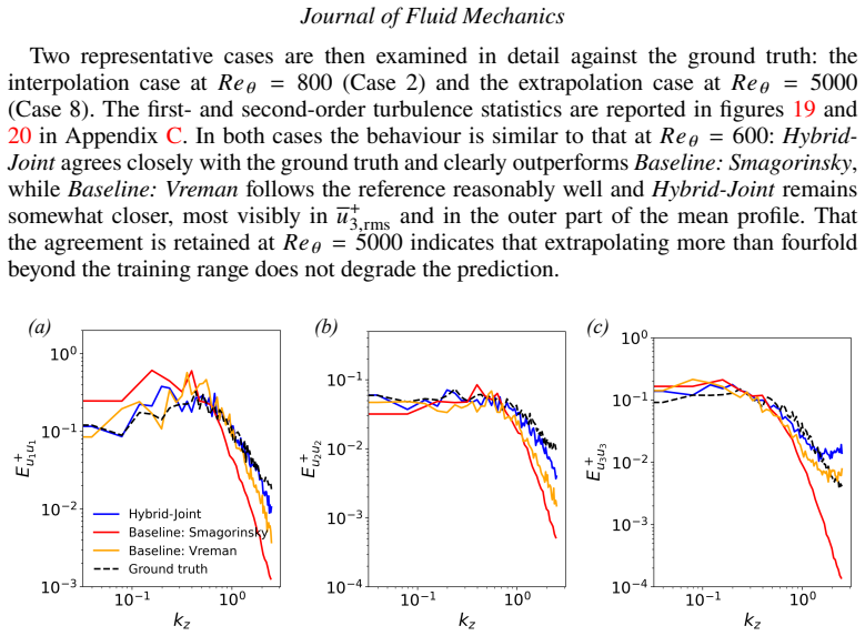
- [§3, Figs. 2, 5, 8, 10] No uncertainty estimates are reported. All statistics are based on single rollouts (final 20 flow-through times), and no ensemble of initial conditions or training runs is shown. Given the chaotic dynamics and the stochastic training procedure, statements such as “agrees closely” and “extrapolates without appreciable degradation” need run-to-run variability or at least a sensitivity study to the averaging window. Without error bars, it is difficult to judge whether Hybrid-Joint’s advantage over Baseline: Vreman in Figs. 2, 8, and 20 is significant relative to natural fluctuations.
- [§3, Case 8 and Appendix C, Fig. 20] The Re_theta = 5000 reference is described in Fig. 20 as “wall-resolved-quality fine-mesh WMLES,” not DNS. This is a model-dependent target, so the claim that Hybrid-Joint “agrees closely” and the quantitative extrapolation assessment are conditional on the fidelity of that reference. Please state explicitly how this reference is validated and, where possible, compare against DNS at overlapping lower Reynolds numbers. The Case 4 reference-domain mismatch is acknowledged in §3.3, but the same caution should be stated for Case 8.
minor comments (5)
- [§2.2.3, Eq. (2.12)] The averaging window T is defined as 10 delta_99 / U_infinity, but delta_99 is not defined before this equation, and the integral upper limit is written as infinity rather than delta_99. Please clarify notation.
- [§3.2, first paragraph] The sentence “This agreement is a genuine test of the model” should be softened or qualified in view of Eq. (2.11), which fixes the mean wall stress and hence the inner scaling. See major comment 1.
- [§3.2, Fig. 5(b)] Because Cf is prescribed by Eq. (2.11), the comparison with Fernholz & Finley data and Smits/Nagib correlations is not independent. Consider plotting the learned correction (Cf_model − Cf_Smits)/Cf_Smits to show what the network actually adds.
- [§4.4, Table 3] The CPU-to-GPU cost comparison is labeled indicative, which is appropriate. However, the claim of a “540× reduction” combines solver efficiency, mesh coarsening, and amortization; this should be broken down more clearly to avoid overstatement.
- [General] No code or data availability statement is included. Given the complexity of the framework, releasing the differentiable solver wrapper and trained weights would materially help reproducibility.
Circularity Check
Extrapolation and skin-friction evidence are largely predetermined by the empirical Smits law and the u_tau anchor; the joint-training conclusion itself is independently supported.
specific steps
-
self definitional
[§2.2.3, Eqs. (2.11)–(2.12); presented as extrapolation evidence in §3.2, Fig. 5(b)]
"Cf = ⟨τ_w,1⟩/(1/2 ρ U∞^2) = 0.024 Re_theta^{-1/4}, ⟨τ_w,3⟩=0 ... The resulting Re_theta is substituted into equation (2.11) to give the reference mean stress."
The mean wall shear stress used by the neural wall closure is prescribed at every time step by the Smits et al. empirical skin-friction law, with Re_theta evaluated online from the running-averaged profile. Therefore the simulated Cf is not an independent output of the learned closures: it is an input of the closure. The paper's claim that the predicted Cf follows the expected Re_theta scaling across 600–6500 is thus largely a restatement of Eq. (2.11), not a test of learned Reynolds-number generalization. The paper itself states this: the scaling law 'provides the correct Re-scaling, which the network need not relearn.'
-
fitted input called prediction
[§2.3, Eq. (2.16); invoked in §3.2 as evidence of accurate inner scaling and extrapolation]
"L(θ) = w1‖⟨u+1⟩−⟨u+1,GT⟩‖^2 + ... + w4‖uτ − uτ,GT‖ ... the final term anchors the absolute magnitude of uτ, which inner scaling alone leaves undetermined."
The friction velocity u_tau is directly included in the training loss, and u_tau is derived from the wall stress produced by the wall closure. Hence the accurate inner-scaled mean profile and the u_tau values at the training Reynolds numbers are fitted quantities, not predictions. At extrapolated Reynolds numbers, the same u_tau is dominated by the prescribed Smits-law mean (Eq. 2.11), so the Reynolds-number trend of the inner scaling is inherited from the empirical law rather than learned. Reporting this agreement as evidence of extrapolation is therefore circular with respect to the training objective.
-
other
[§4.1.2, Fig. 16]
"The mean-only model gives a reasonable, slightly overpredicted mean velocity profile, since the imposed mean wall stress still provides the correct inner scaling."
This ablation explicitly shows that the reasonable mean velocity profile — the basis for the log-region and inner-scaling claims — is obtained even when the learned wall-stress fluctuations are removed, because the mean wall stress is imposed by the scaling law. It confirms that the mean-profile agreement is not produced by the learned correction but by the empirical input. The learned fluctuations are needed for the Reynolds shear stress, which is genuine, but the mean-profile and Cf-based extrapolation evidence is tied to the prescribed input.
full rationale
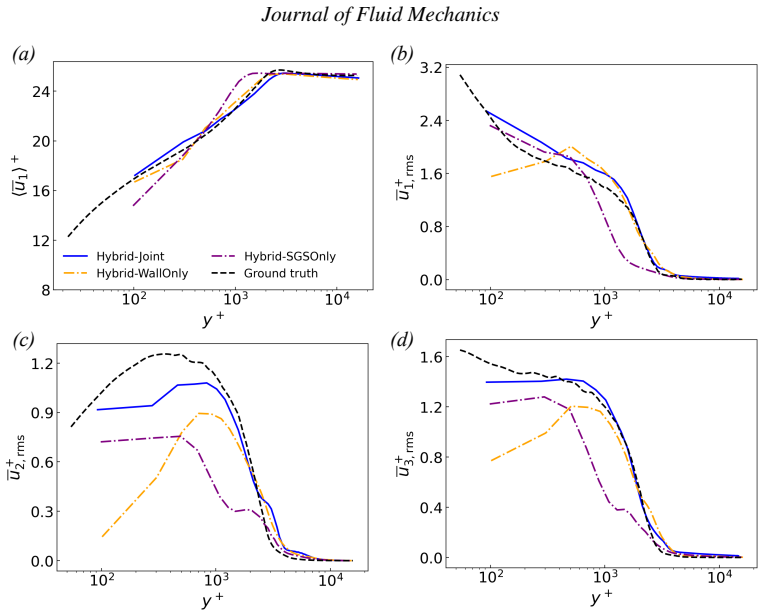
The paper's central methodological claim — that the SGS closure, wall closure, and discretization are coupled and must be trained jointly — is independently supported by the ablation experiments (Hybrid-WallOnly and Hybrid-SGSOnly fail in complementary ways), and several reported results are genuinely emergent: the SGS coefficient near c≈0.07, the resolved spectra, the wall-stress fluctuation PDFs, and the need for fluctuations to recover the Reynolds shear stress. However, the Reynolds-number extrapolation claim is substantially prebuilt. The mean wall stress is set by the Smits et al. skin-friction law (Eq. 2.11) with online Re_theta (Eq. 2.12), and the loss contains an explicit u_tau anchor (Eq. 2.16). Consequently, the Cf–Re_theta agreement, the inner-scaled mean profile, and the log-region behavior at extrapolated Reynolds numbers are not independent tests of a learned Reynolds-number-scaling law; they largely reflect the empirical input plus a small trained correction. The paper openly acknowledges that the scaling law 'provides the correct Re-scaling, which the network need not relearn', and the mean-only ablation corroborates that the mean profile is reasonable even without the learned fluctuation. This is partial circularity in the generalization evidence, not in the joint-optimization conclusion, so a score of 6 is appropriate rather than higher.
Axiom & Free-Parameter Ledger
free parameters (6)
- Neural SGS U-Net weights (θ_sgs) =
trained (architecture in Table 4)
- Neural wall U-Net weights (θ_wall) =
trained (architecture in Table 4)
- Smits et al. skin-friction law constants (0.024, -1/4) =
0.024 Re_theta^-1/4
- Training Reynolds number set =
{600, 1200}
- Momentum-thickness averaging window T =
10 δ99/U∞
- Loss weights w_k = 1/|L_k| =
recomputed per epoch, detached
axioms (7)
- domain assumption Filtered incompressible Navier-Stokes equations (2.1) govern the resolved field with implicit filtering by the mesh
- domain assumption Eddy-viscosity form for SGS stress, τ_ij = -2ν_t S_ij
- domain assumption Vreman functional (2.7)-(2.8) as fixed output layer remains a suitable tensor structure for the learned coefficient
- domain assumption Empirical skin-friction law of Smits et al. (2.11) gives accurate mean wall shear stress
- domain assumption Local resolved fields at the third off-wall cell contain enough information for the wall network to predict stress fluctuations
- domain assumption Statistics accumulated over the final 20 flow-through times are converged without error bars
- domain assumption Recycling-rescaling inflow (Lund et al. 1998) provides sufficient turbulence for autonomous transition and development
Cite this review
Pith. "Pith review of Differentiable Hybrid Neural-CFD Modelling of Wall-Bounded Turbulence: Coupled Learning of Subgrid-Scale and Wall Closures." pith.science (2026). https://pith.science/paper/DRTRBBPE
@misc{pith2026260717357,
  author       = {Pith},
  title        = {Pith review of: Differentiable Hybrid Neural-CFD Modelling of Wall-Bounded Turbulence: Coupled Learning of Subgrid-Scale and Wall Closures},
  year         = {2026},
  howpublished = {\url{https://pith.science/paper/DRTRBBPE}},
  note         = {Machine review of arXiv:2607.17357}
}
read the original abstract
Wall-modelled large-eddy simulation (WMLES) treats the subgrid-scale (SGS) closure, wall closure and numerical discretization as independent components, although their effects are coupled through the same resolved field. We present a differentiable hybrid neural--CFD framework in which the SGS and wall closures are learned jointly, end-to-end, within a differentiable flow solver, using only low-order statistics as training targets. Each closure is a composed neural operator: a trainable neural network followed by a fixed differentiable layer that preserves the structure of its conventional counterpart, so that the network learns only the functions left undetermined by the conventional form. Because every operation is differentiable, gradients of the training loss are back-propagated through the coupled solver, allowing both neural closures to be optimized consistently against the flow field, rather than fitted offline or in isolation. We demonstrate the framework, denoted Hybrid-Joint, on a zero-pressure-gradient turbulent boundary layer across a posteriori tests spanning Re_\theta = 600--6500, computational domains and mesh resolutions. The model outperforms WMLES baselines, extrapolates to more than four times the highest training Reynolds number, and transfers to grids and domains absent from training. It recovers a logarithmic mean-velocity region, not imposed by the wall closure, and reproduces the resolved energy spectra accurately, although spectral information is excluded from the training objective. Ablation studies show that learning either closure alone is insufficient and that only joint optimization recovers the full set of statistics, confirming that SGS closure, wall closure and discretization are coupled and must be trained jointly. Once trained, the closures are reused without retraining across all cases, so that training cost is amortized over repeated deployment.
Figures






Reference graph
Works this paper leans on
-
[1]
Physics of Fluids 27 (3)
Abkar, Mahdi & Port \'e -Agel, Fernando 2015 Influence of atmospheric stability on wind-turbine wakes: A large-eddy simulation study . Physics of Fluids 27 (3)
2015
-
[2]
Theoretical and Applied Mechanics Letters p
Akhare, Deepak , Luo, Tengfei & Wang, Jian-Xun 2025 HybridNDiff-UQ : Uncertainty quantification for hybrid neural differentiable modeling . Theoretical and Applied Mechanics Letters p. 100609
2025
-
[3]
Fluids 6 (3), 112
Bae, H Jane & Lozano-Dur \'a n, Adri \'a n 2021 Effect of wall boundary conditions on a wall-modeled large-eddy simulation in a finite-difference framework . Fluids 6 (3), 112
2021
-
[4]
In 13th Fluid and Plasmadynamics Conference\/ , p
Bardina, Jorge , Ferziger, J & Reynolds, WC 1980 Improved subgrid-scale models for large-eddy simulation. In 13th Fluid and Plasmadynamics Conference\/ , p. 1357
1980
-
[5]
Computer Physics Communications 282 , 108527
Bezgin, Deniz A , Buhendwa, Aaron B & Adams, Nikolaus A 2023 Jax-fluids: A fully-differentiable high-order computational fluid dynamics solver for compressible two-phase flows . Computer Physics Communications 282 , 108527
2023
-
[6]
Annual Review of Fluid Mechanics 50 , 535--561
Bose, Sanjeeb T & Park, George Ilhwan 2018 Wall-modeled large-eddy simulation for complex turbulent flows . Annual Review of Fluid Mechanics 50 , 535--561
2018
-
[7]
2021 Integral measures of the zero pressure gradient boundary layer over the R eynolds number range 0 R_ <
Cantwell, Brian J. 2021 Integral measures of the zero pressure gradient boundary layer over the R eynolds number range 0 R_ < . Physics of Fluids 33 (8), 085108
2021
-
[8]
AIAA Journal 17 (12), 1293--1313
Chapman, Dean R 1979 Computational aerodynamics development and outlook . AIAA Journal 17 (12), 1293--1313
1979
-
[9]
Journal of Fluid Mechanics 1024 , A28
Chedevergne, Fran c ois 2025 Characterisation and modelling of interscale energy transfers in high R eynolds number boundary layers . Journal of Fluid Mechanics 1024 , A28
2025
-
[10]
Journal of Fluid Mechanics 91 (1), 1--16
Clark, Robert A , Ferziger, Joel H & Reynolds, William Craig 1979 Evaluation of subgrid-scale models using an accurately simulated turbulent flow . Journal of Fluid Mechanics 91 (1), 1--16
1979
-
[11]
arXiv preprint arXiv:2603.15920
Du, Pan , Li, Yongqi , Xu, Mingqi & Wang, Jian-Xun 2026 DiFVM : A vectorized graph-based finite volume solver for differentiable cfd on unstructured meshes . arXiv preprint arXiv:2603.15920
arXiv 2026
-
[12]
Annual Review of Fluid Mechanics 51 (1), 357--377
Duraisamy, Karthik , Iaccarino, Gianluca & Xiao, Heng 2019 Turbulence modeling in the age of data . Annual Review of Fluid Mechanics 51 (1), 357--377
2019
-
[13]
Physics of Fluids 37 (9)
Fan, Guoqing , Zhao, Weiwen & Wan, Decheng 2025 a\/ Near-wall turbulent fluctuations and coherent structures in wall-modeled large-eddy simulation . Physics of Fluids 37 (9)
2025
-
[14]
Computer Methods in Applied Mechanics and Engineering 433 , 117478
Fan, Xiantao , Akhare, Deepak & Wang, Jian-Xun 2025 b\/ Neural differentiable modeling with diffusion-based super-resolution for two-dimensional spatiotemporal turbulence . Computer Methods in Applied Mechanics and Engineering 433 , 117478
2025
-
[15]
Computer Methods in Applied Mechanics and Engineering 448 , 118455
Fan, Xiantao , Liu, Xin-Yang , Wang, Meng & Wang, Jian-Xun 2026 Diff-FlowFSI : A GPU -optimized differentiable CFD platform for high-fidelity turbulence and FSI simulations . Computer Methods in Applied Mechanics and Engineering 448 , 118455
2026
-
[16]
Journal of Computational Physics 496 , 112584
Fan, Xiantao & Wang, Jian-Xun 2024 Differentiable hybrid neural modeling for fluid-structure interaction . Journal of Computational Physics 496 , 112584
2024
-
[17]
Progress in Aerospace Sciences 32 (4), 245--311
Fernholz, Hans-Hermann & Finley, PJ 1996 The incompressible zero-pressure-gradient turbulent boundary layer: an assessment of the data . Progress in Aerospace Sciences 32 (4), 245--311
1996
-
[18]
Journal of Fluid Mechanics 934 , A44
Fowler, Mitchell , Zaki, Tamer A & Meneveau, Charles 2022 A lagrangian relaxation towards equilibrium wall model for large eddy simulation . Journal of Fluid Mechanics 934 , A44
2022
-
[19]
Journal of Computational Physics p
Franz, Aleksandra , Wei, Hao , Guastoni, Luca & Thuerey, Nils 2025 PICT --a differentiable, GPU -accelerated multi-block PISO solver for simulation-coupled learning tasks in fluid dynamics . Journal of Computational Physics p. 114433
2025
-
[20]
Physical Review Fluids 4 (6), 064603
Fukami, Kai , Nabae, Yusuke , Kawai, Ken & Fukagata, Koji 2019 Synthetic turbulent inflow generator using machine learning . Physical Review Fluids 4 (6), 064603
2019
-
[21]
Physics of Fluids A: Fluid dynamics 3 (7), 1760--1765
Germano, Massimo , Piomelli, Ugo , Moin, Parviz & Cabot, William H 1991 A dynamic subgrid-scale eddy viscosity model . Physics of Fluids A: Fluid dynamics 3 (7), 1760--1765
1991
-
[22]
Journal of Computational Physics 458 , 111090
Guan, Yifei , Chattopadhyay, Ashesh , Subel, Adam & Hassanzadeh, Pedram 2022 Stable a posteriori LES of 2D turbulence using convolutional neural networks: Backscattering analysis and generalization to higher R e via transfer learning . Journal of Computational Physics 458 , 111090
2022
-
[23]
Journal of Fluid Mechanics 928 , A27
Guastoni, Luca , G \"u emes, Alejandro , Ianiro, Andrea , Discetti, Stefano , Schlatter, Philipp , Azizpour, Hossein & Vinuesa, Ricardo 2021 Convolutional-network models to predict wall-bounded turbulence from wall quantities . Journal of Fluid Mechanics 928 , A27
2021
-
[24]
Physical Review Fluids 11 (1), 014602
Huang, Xinyi , Leung, Sze Chai & Bae, H Jane 2026 Consistency requirement of data-driven subgrid-scale modeling in large-eddy simulation . Physical Review Fluids 11 (1), 014602
2026
-
[25]
Physics of Fluids 24 (1)
Kawai, Soshi & Larsson, Johan 2012 Wall-modeling in large eddy simulation: Length scales, grid resolution, and accuracy . Physics of Fluids 24 (1)
2012
-
[26]
Kim, Hojin , Shankar, Varun , Viswanathan, Venkatasubramanian & Maulik, Romit 2025 Generalizable data-driven turbulence closure modeling on unstructured grids with differentiable physics, arXiv:arXiv: 2307.13533
arXiv 2025
-
[27]
Proceedings of the National Academy of Sciences 118 (21), e2101784118
Kochkov, Dmitrii , Smith, Jamie A , Alieva, Ayya , Wang, Qing , Brenner, Michael P & Hoyer, Stephan 2021 Machine learning--accelerated computational fluid dynamics . Proceedings of the National Academy of Sciences 118 (21), e2101784118
2021
-
[28]
Neural Networks p
Kohl, Georg , Chen, Li-Wei & Thuerey, Nils 2026 Benchmarking autoregressive conditional diffusion models for turbulent flow simulation . Neural Networks p. 108641
2026
-
[29]
Mechanical Engineering Reviews 3 (1), 15--00418
Larsson, Johan , Kawai, Soshi , Bodart, Julien & Bermejo-Moreno, Ivan 2016 Large eddy simulation with modeled wall-stress: recent progress and future directions . Mechanical Engineering Reviews 3 (1), 15--00418
2016
-
[30]
Physics of Fluids 35 (7)
Li, Zhijie , Peng, Wenhui , Yuan, Zelong & Wang, Jianchun 2023 Long-term predictions of turbulence by implicit U - N et enhanced f o urier neural operator . Physics of Fluids 35 (7)
2023
-
[31]
NCAR Report
Lilly, D 1966 On the application of the eddy viscosity concept in the inertial sub-range of turbulence . NCAR Report
1966
-
[32]
In AIAA SCITECH 2025 Forum\/ , p
Ling, Yuenong & Lozano-Duran, Adrian 2025 Numerically consistent data-driven subgrid-scale model via data assimilation and machine learning. In AIAA SCITECH 2025 Forum\/ , p. 1280
2025
-
[33]
Computer Methods in Applied Mechanics and Engineering 433 , 117441
List, Bjoern , Chen, Li-Wei , Bali, Kartik & Thuerey, Nils 2025 Differentiability in unrolled training of neural physics simulators on transient dynamics . Computer Methods in Applied Mechanics and Engineering 433 , 117441
2025
-
[34]
Journal of Fluid Mechanics 949 , A25
List, Bj \"o rn , Chen, Li-Wei & Thuerey, Nils 2022 Learned turbulence modelling with differentiable fluid solvers: physics-based loss functions and optimisation horizons . Journal of Fluid Mechanics 949 , A25
2022
-
[35]
Journal of computational physics 140 (2), 233--258
Lund, Thomas S , Wu, Xiaohua & Squires, Kyle D 1998 Generation of turbulent inflow data for spatially-developing boundary layer simulations . Journal of computational physics 140 (2), 233--258
1998
-
[36]
Physical Review Fluids 6 (5), 050502
MacArt, Jonathan F , Sirignano, Justin & Freund, Jonathan B 2021 Embedded training of neural-network subgrid-scale turbulence models . Physical Review Fluids 6 (5), 050502
2021
-
[37]
Journal of Fluid Mechanics 858 , 122--144
Maulik, Romit , San, Omer , Rasheed, Adil & Vedula, Prakash 2019 Subgrid modelling for two-dimensional turbulence using neural networks . Journal of Fluid Mechanics 858 , 122--144
2019
-
[38]
Scientific Data 8 (1), 255
McConkey, Ryley , Yee, Eugene & Lien, Fue-Sang 2021 A curated dataset for data-driven turbulence modelling . Scientific Data 8 (1), 255
2021
-
[39]
Annual Review of Fluid Mechanics 32 (1), 1--32
Meneveau, Charles & Katz, Joseph 2000 Scale-invariance and turbulence models for large-eddy simulation . Annual Review of Fluid Mechanics 32 (1), 1--32
2000
-
[40]
Physical Review Fluids 6 (10), 104607
Mons, Vincent , Du, Yifan & Zaki, Tamer A 2021 Ensemble-variational assimilation of statistical data in large-eddy simulation . Physical Review Fluids 6 (10), 104607
2021
-
[41]
Journal of Fluid Mechanics 1003 , A2
Nabae, Yusuke , Inagaki, Kazuhiro , Kobayashi, Hiromichi , Gotoda, Hiroshi & Fukagata, Koji 2025 Large-eddy simulation of high- R eynolds-number turbulent channel flow controlled using streamwise travelling wave-like wall deformation for drag reduction . Journal of Fluid Mechanics 1003 , A2
2025
-
[43]
PhD thesis, Stanford University
Piomelli, Ugo 1988 Models for large eddy simulations of turbulent channel flows including transpiration . PhD thesis, Stanford University
1988
-
[44]
Progress in Aerospace Sciences 44 (6), 437--446
Piomelli, Ugo 2008 Wall-layer models for large-eddy simulations . Progress in Aerospace Sciences 44 (6), 437--446
2008
-
[45]
Annual Review of Fluid Mechanics 34 (1), 349--374
Piomelli, Ugo & Balaras, Elias 2002 Wall-layer models for large-eddy simulations . Annual Review of Fluid Mechanics 34 (1), 349--374
2002
-
[46]
International Journal of Heat and Fluid Flow 24 (4), 538--550
Piomelli, Ugo , Balaras, Elias , Pasinato, Hugo , Squires, Kyle D & Spalart, Philippe R 2003 The inner--outer layer interface in large-eddy simulations with wall-layer models . International Journal of Heat and Fluid Flow 24 (4), 538--550
2003
-
[47]
Physics of Fluids A: Fluid Dynamics 3 (7), 1766--1771
Piomelli, Ugo , Cabot, William H , Moin, Parviz & Lee, Sangsan 1991 Subgrid-scale backscatter in turbulent and transitional flows . Physics of Fluids A: Fluid Dynamics 3 (7), 1766--1771
1991
-
[48]
Physics of Fluids 8 (1), 215--224
Piomelli, Ugo , Yu, Yunfang & Adrian, Ronald J 1996 Subgrid-scale energy transfer and near-wall turbulence structure . Physics of Fluids 8 (1), 215--224
1996
-
[49]
Journal of Fluid Mechanics 415 , 261--284
Port \'e -Agel, Fernando , Meneveau, Charles & Parlange, Marc B 2000 A scale-dependent dynamic model for large-eddy simulation: application to a neutral atmospheric boundary layer . Journal of Fluid Mechanics 415 , 261--284
2000
-
[50]
Computers & Fluids 185 , 34--58
Rezaeiravesh, Saleh , Mukha, Timofey & Liefvendahl, Mattias 2019 Systematic study of accuracy of wall-modeled large eddy simulation using uncertainty quantification techniques . Computers & Fluids 185 , 34--58
2019
-
[51]
Journal of Fluid Mechanics 659 , 116--126
Schlatter, Philipp & \"O rl \"u , Ramis 2010 Assessment of direct numerical simulation data of turbulent boundary layers . Journal of Fluid Mechanics 659 , 116--126
2010
-
[52]
Physical Review Fluids 10 (2), 024605
Shankar, Varun , Chakraborty, Dibyajyoti , Viswanathan, Venkatasubramanian & Maulik, Romit 2025 Differentiable turbulence: Closure as a partial differential equation constrained optimization . Physical Review Fluids 10 (2), 024605
2025
-
[53]
Journal of Fluid Mechanics 966 , A26
Sirignano, Justin & MacArt, Jonathan F 2023 Deep learning closure models for large-eddy simulation of flows around bluff bodies . Journal of Fluid Mechanics 966 , A26
2023
-
[54]
the basic experiment
Smagorinsky, Joseph 1963 General circulation experiments with the primitive equations: I. the basic experiment . Monthly Weather Review 91 (3), 99--164
1963
-
[55]
Journal of Ship Research 27 (03), 147--157
Smits, AJ , Matheson, N & Joubert, PN 1983 Low- R eynolds-number turbulent boundary layers in zero and favorable pressure gradients . Journal of Ship Research 27 (03), 147--157
1983
-
[56]
International Journal of Heat and Fluid Flow 26 (2), 173--190
Temmerman, L , Had z iabdi \'c , M , Leschziner, MA & Hanjali \'c , K 2005 A hybrid two-layer URANS -- LES approach for large eddy simulation at high R eynolds numbers . International Journal of Heat and Fluid Flow 26 (2), 173--190
2005
-
[57]
International Journal of Heat and Fluid Flow 27 (5), 789--799
Tessicini, F , Temmerman, L & Leschziner, MA 2006 Approximate near-wall treatments based on zonal and hybrid RANS -- LES methods for LES at high R eynolds numbers . International Journal of Heat and Fluid Flow 27 (5), 789--799
2006
-
[58]
Journal of the Aeronautical Sciences 23 (11), 1007--1011
Van Driest, Edward R 1956 On turbulent flow near a wall . Journal of the Aeronautical Sciences 23 (11), 1007--1011
1956
-
[59]
Physics of Fluids 16 (10), 3670--3681
Vreman, AW 2004 An eddy-viscosity subgrid-scale model for turbulent shear flow: Algebraic theory and applications . Physics of Fluids 16 (10), 3670--3681
2004
-
[60]
Physical Review Fluids 2 (3), 034603
Wang, Jian-Xun , Wu, Jin-Long & Xiao, Heng 2017 Physics-informed machine learning approach for reconstructing reynolds stress modeling discrepancies based on DNS data . Physical Review Fluids 2 (3), 034603
2017
-
[61]
Journal of Computational Physics 267 , 210--224
Wang, Qiqi , Hu, Rui & Blonigan, Patrick 2014 Least squares shadowing sensitivity analysis of chaotic limit cycle oscillations . Journal of Computational Physics 267 , 210--224
2014
-
[62]
Wang, Qi , Wang, Mengze & Zaki, Tamer A 2022 What is observable from wall data in turbulent channel flow? Journal of Fluid Mechanics 941 , A48
2022
-
[63]
Journal of Fluid Mechanics 906 , A14
Wang, Wenkang , Pan, Chong & Wang, Jinjun 2021 Energy transfer structures associated with large-scale motions in a turbulent boundary layer . Journal of Fluid Mechanics 906 , A14
2021
-
[64]
& Font, B
Weymouth, G.D. & Font, B. 2025 Water L ily.jl: A differentiable and backend-agnostic J ulia solver for incompressible viscous flow around dynamic bodies . Computer Physics Communications 315 , 109748
2025
-
[66]
Journal of Fluid Mechanics 869 , 553--586
Wu, Jinlong , Xiao, Heng , Sun, Rui & Wang, Qiqi 2019 Reynolds-averaged N avier-- S tokes equations with explicit data-driven reynolds stress closure can be ill-conditioned . Journal of Fluid Mechanics 869 , 553--586
2019
-
[67]
Physical Review Fluids 4 (3), 034602
Yang, XIA , Zafar, S , Wang, J-X & Xiao, H 2019 Predictive large-eddy-simulation wall modeling via physics-informed neural networks . Physical Review Fluids 4 (3), 034602
2019
-
[68]
Physics of Fluids 33 (1)
Yang, Xiang IA & Griffin, Kevin P 2021 Grid-point and time-step requirements for direct numerical simulation and large-eddy simulation . Physics of Fluids 33 (1)
2021
-
[69]
Physical Review Fluids 2 (10), 104601
Yang, Xiang IA , Park, George Ilhwan & Moin, Parviz 2017 Log-layer mismatch and modeling of the fluctuating wall stress in wall-modeled large-eddy simulations . Physical Review Fluids 2 (10), 104601
2017
-
[70]
Journal of Computational Physics p
Zhang, Fengshun , Yang, Xiaolei & He, Guowei 2026 A differentiable wall-modeled large-eddy simulation method for high- R eynolds-number wall-bounded turbulent flows . Journal of Computational Physics p. 114835
2026
-
[71]
Journal of Fluid Mechanics 949 , A26
Zhang, Xin-Lei , Xiao, Heng , Luo, Xiaodong & He, Guowei 2022 Ensemble K alman method for learning turbulence models from indirect observation data . Journal of Fluid Mechanics 949 , A26
2022
-
[72]
Journal of Computational Physics 506 , 112948
Zhou, Di & Bae, H Jane 2024 Sensitivity analysis of wall-modeled large-eddy simulation for separated turbulent flow . Journal of Computational Physics 506 , 112948
2024
-
[74]
Physical Review Fluids , volume=
Differentiable turbulence: Closure as a partial differential equation constrained optimization , author=. Physical Review Fluids , volume=. 2025 , publisher=
2025
-
[75]
Physical Review Fluids , volume=
Synthetic turbulent inflow generator using machine learning , author=. Physical Review Fluids , volume=. 2019 , publisher=
2019
-
[76]
Neural Networks , pages=
Benchmarking autoregressive conditional diffusion models for turbulent flow simulation , author=. Neural Networks , pages=. 2026 , publisher=
2026
-
[77]
Physics of Fluids , volume=
An eddy-viscosity subgrid-scale model for turbulent shear flow: Algebraic theory and applications , author=. Physics of Fluids , volume=. 2004 , publisher=
2004
-
[78]
Physics of Fluids , volume=
A dynamic subgrid-scale eddy viscosity model with a global model coefficient , author=. Physics of Fluids , volume=. 2006 , publisher=
2006
-
[79]
Physics of Fluids , volume=
A dynamic global-coefficient subgrid-scale eddy-viscosity model for large-eddy simulation in complex geometries , author=. Physics of Fluids , volume=. 2007 , publisher=
2007
-
[80]
The basic experiment , author=
General circulation experiments with the primitive equations: I. The basic experiment , author=. Monthly Weather Review , volume=
-
[81]
Physics of Fluids A: Fluid dynamics , volume=
A dynamic subgrid-scale eddy viscosity model , author=. Physics of Fluids A: Fluid dynamics , volume=. 1991 , publisher=
1991
-
[82]
Meneveau, Charles and Lund, Thomas S and Cabot, William H , journal=. A. 1996 , publisher=
1996
-
[83]
Fluids , volume=
Effect of wall boundary conditions on a wall-modeled large-eddy simulation in a finite-difference framework , author=. Fluids , volume=. 2021 , publisher=
2021
This paper was first reviewed by deepseek-v4-flash on August 1, 2026.
discussion (0)
Sign in with ORCID, Apple, or X to comment. Anyone can read and Pith papers without signing in.