REVIEW 3 major objections 4 minor 64 references
Noise structuring in fixed-depth Trotter simulation: stationary channels and observable-level depolarization
T0 review · 3 major / 4 minor · reviewed 2026-08-01 · deepseek-v4-flash
Pith's one-line read Fixed-depth Trotter circuits convert local hardware noise into a stationary, endpoint-independent noise channel after a crossover time, so observable dynamics are recovered by a single affine contrast correction.
desk verdict Worth refereeing: the fixed-depth noise-structuring idea is new and useful, but the central factorization lacks a quantified error bound at the advertised crossover. read the letter →
The pith
A machine-rendered reading of the paper's core claim, the machinery that carries it, and where it could break.
The reading
What carries the argument
The key object is the single-fault channel M_ξ(T) = (1/T)∫_0^T dt P_ξ(−t) ρ P_ξ(−t), where P_ξ(−t) is the Pauli fault propagated to the toggling frame by the ideal dynamics. After a memory time T* (diagnosed by a Loschmidt echo of the local perturbation δE = P_ξ H P_ξ − H), this channel converges to a stationary limit M_ξ, which then commutes with the ideal evolution. Averaging M_ξ over fault patterns gives M, and combining independent faulty layers yields the binomial channel [(1−q)I + q M]^N, with the Poissonian exponential exp[μ(M−I)] as its dilute-layer limit. This factorization is what converts time-dependent microscopic noise into an endpoint-independent, low-dimensional correction.
What would settle it
For a fixed-depth circuit using a CNOT-heavy transpilation known to produce long propagated Pauli strings, compute the diamond-norm distance between the actual noisy channel and [(1−q)I+qM]^N∘U(T) as a function of T. If this distance does not fall to zero for T ≳ μT*, the claimed factorization fails. Alternatively, fit the affine coefficients a_O and c_O in two non-overlapping late-time windows and check whether they agree within shot noise; disagreement would indicate that the stationary observable-level rescaling is not actually endpoint-independent.
Extended reading notes
Core claim
The central discovery is that, for fixed-depth Trotter circuits with local stochastic Pauli faults, the full noisy channel factorizes as Q_N(T) ≃ [(1−q)I + q M]^N ∘ U(T) once T is larger than a memory-loss scale T_stat = μT*. Here M is the stationary single-fault channel averaged over fault patterns, and U(T) is the ideal evolution. In the dilute-layer limit q→0 with μ = Nq fixed, this becomes exp[μ(M−I)] ∘ U(T). Because M commutes with the ideal dynamics, the noise channel can be moved to the end of the circuit and acts as a stationary dressing. At the observable level, the channel's action is well approximated by an affine map, ⟨O⟩_noisy(T) ≃ a_O(N,q)⟨O⟩_ideal(T) + c_O(N,q), valid for T ≳
Load-bearing premise
The central claim collapses if the dominant Pauli faults stop being local—for instance, when a CNOT cascade turns a single local error into a long Pauli string—because then the propagated single-fault channel no longer converges to a stationary endpoint-independent channel on the relevant timescales.
Editorial extensions
If this is right
- After the stationary crossover, one contrast factor and one offset per observable suffice to reconstruct ideal dynamics over an extended time window, making noise calibration a one-time procedure.
- The dilute-layer Poissonian channel provides a microscopic justification for global-folding zero-noise extrapolation, with the same stationary channel amplified by the expected 2n+1 factor.
- The crossover time T_stat separates two error-mitigation complexity regimes: below it a single-exponential ZNE fit fails and can produce unphysical values, while above it a single-mode approximation becomes accurate.
- Higher-order Trotter decompositions broaden the consistency window in which the stationary-channel description applies, at the cost of a potentially larger layer error probability q.
- The binomial channel, not the Poisson exponential, is the correct finite-depth expression; the two differ at order μq, which matters when noise is not dilute.
Reading between the lines
- The locality assumption suggests that hardware with native two-qubit interactions (e.g., RZZ or RZX gates) is more naturally compatible with this stationary-channel picture than CNOT-heavy layouts, and this could be tested by comparing the crossover behavior on devices with different transpilations.
- The digital Zeno-like transient, though presented as a failure regime, could be repurposed as a calibration signal: its onset time directly estimates μT*, giving a noise-aware measure of the effective depolarization rate on a device.
- The spectral criterion μ²W² ≲ 1 derived in the paper could be used as a pre-simulation check to predict when observable-level depolarization will hold, potentially saving calibration effort before running an expensive time scan.
- If the stationary-channel claim extends to non-dilute regimes (q close to 1), a local space-time fault-density formulation would be required; the paper itself points to this as an open direction.
Editorial analysis
A structured set of objections, weighed in public.
Referee Report
Summary. The paper analyzes fixed-depth Trotter simulation as a noise-structuring protocol. With the number of Trotter layers fixed by the largest endpoint time, the total hardware-noise dose becomes approximately endpoint-independent. For local stochastic Pauli faults, the authors argue that after propagated faults lose memory of their insertion layer, the noisy circuit factorizes into the ideal evolution followed by a stationary finite-depth binomial channel, Eq. (34); in the dilute-layer limit this becomes a Poissonian exponential. The single-fault memory time is related to a Loschmidt echo. The practical corollary is observable-level depolarization: for selected observables and moderate noise, the stationary channel acts as an almost time-independent affine contrast correction, Eq. (43), which is proposed as a basis for error mitigation. The paper also describes a digital Zeno-like short-time transient and discusses implications for zero-noise extrapolation.
Significance. The fixed-depth protocol is a plausible and practically motivated alternative to standard fixed-step and fixed-error scans, and the claimed channel factorization would provide a useful microscopic justification for affine rescaling and global-folding ZNE in Trotterized simulations. The paper is careful to separate coherent Trotter error from hardware noise, and it supplies analytic machinery (single-fault channels, Loschmidt-echo memory times, ordered-sum derivations, spectral bounds) as well as numerical illustrations for a small transverse-field Ising chain. Machine-readable data and code are promised via Zenodo. However, the central factorization is not yet quantitatively controlled, and the observable-level affine rescaling relies on additional unproven spectral-concentration assumptions. The significance is therefore real but conditional on closing the technical gaps below.
major comments (3)
- [Appendix B3; Eq. (34)] The central factorization is not quantitatively controlled. The recursive identity (B35)-(B38) shows only that, under the induction hypothesis, an averaged single-fault insertion with time distributed over [0,T] yields M_xi_i in the limit T/M -> infinity. It does not bound the error when insertions lie close to boundaries or to one another. At the advertised crossover Tstat ~ mu T* with typical M ~ mu, the condition T/M ≳ T* is only marginal; the 'exceptional regions' of the simplex have relative volume that the paper asserts is small but does not estimate. Since Appendix B2 gives an exact expression for the single-fault mismatch Delta M(T) in Eq. (B25), an explicit bound of the form ||I_M - product_i M_xi_i|| <= C_M [sum_i Delta M(T/M)] plus boundary terms should be derived and summed over the binomial distribution. Without such an estimate, Eqs. (34), (39)-(43) inherit an uncontrolled
- [Section V, Eq. (40); Appendix B5] The observable-level affine rescaling is asserted rather than derived. The spectral bound in Appendix B5 controls only the normalized Frobenius distance between E_bin and a fully depolarizing channel via the second moment m2(M); the step from such a global bound to a single observable's affine rescaling, Eq. (42), relies on the unproved statement that 'there is no mechanism that concentrates the elements of the R operator solely in the Bohr-diagonal sector' and on treating the inequality as 'qualitatively closer to a ≪ bound.' For the practical claim Eq. (43), an explicit error estimate depending on the observable O and the state rho is needed, for example a bound on the residual ||E_bin(O) - [a_O <O>_ideal + c_O]|| over the claimed time window. As written, the numerical evidence for Eq. (43) is suggestive but not conclusive.
- [Appendix A, Eq. (A6)] The locality assumption is load-bearing and not guaranteed for CNOT-based compilations. The text explicitly notes that CNOT transpilations with long cascades can turn a local Pauli error into a long string, which invalidates the Loschmidt-echo and stationary-channel argument. Since the main text's example uses first-order Trotterization with CNOT transpilation, the paper should either provide a concrete criterion or diagnostic to verify supp P_xi = O(1) and ||v_xi|| <= v_max for a given circuit, or explicitly restrict the central claim to native RZZ/RZX layouts. As it stands, the applicability of Eq. (34) to standard superconducting two-qubit gate compilations is unclear.
minor comments (4)
- [Abstract and Introduction] Numerous typos should be corrected: 'crusial', 'extrapolatin', 'buttomakethe', 'achive', 'ovversimplified', 'foldind' in Section V, and similar errors throughout.
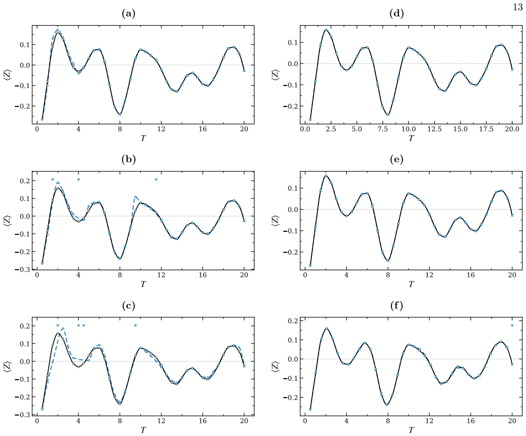
- [Fig. 2 caption] The caption states that the second column uses 'an optimally chosen number of exponents' but the selection procedure is not described. Please specify how the number of exponents was chosen, or label the plot as illustrative.
- [Section V, Eq. (40)] The weights \tilde w_P are used in Eq. (40) before their definition in the following paragraph. Reorder the text so that the definition precedes the equation.
- [Appendix B4, Eq. (B46)] The finite-depth correction in Eq. (37) is stated as O(sqrt(n_O/n_loc)), but the derivation leading to this specific form is not shown. A short derivation or a reference to the appendix equations would help.
Circularity Check
No significant circularity: the central factorization is derived from the microscopic error model; minor self-citations are contextual, not load-bearing.
full rationale
The central chain runs from the local stochastic Pauli model (Eqs. (5)-(9)) to the single-fault channel M_xi^(T) in Eq. (26), its stationary limit (Appendix B2), and the fixed-M ordered-sum factorization (Appendix B3, Eqs. (B35)-(B44)), yielding the binomial channel E_bin in Eq. (34). None of these steps assumes the affine observable-level result Eq. (43) or uses a_O, c_O as input. Instead, the affine rescaling is presented as a later observable-level approximation justified by spectral concentration (Appendix B5), with coefficients explicitly meant to be calibrated: 'The coefficients aO and cO may be obtained from calibration circuits...'. The paper also openly flags the locality restriction (Appendix A.1, Eq. (A6)) and notes that the ordered-sum replacement in Appendix B3 is controlled only under T/M ≳ T*, with exceptional simplex regions having small relative volume; this is a rigor/correctness limitation, not definitional circularity. Self-citations such as [29] document prior observation of similar rescaling behavior, but Eq. (34) is derived from the error model and unitary propagation, not imported from those papers. No load-bearing self-citation or constructional equivalence was found; the score reflects only the presence of minor, non-load-bearing self-citations.
Assumptions & free parameters
free parameters (3)
- T* (single-fault memory time) =
not specified; estimated as ~1/σ_z under a Gaussian approximation, otherwise model-dependent
- a_O (observable contrast factor) =
not predicted; obtained by calibration or ZNE fit
- c_O (affine offset) =
not predicted; obtained by calibration
assumptions (6)
- domain assumption Local stochastic depolarizing noise after each elementary gate (Eq. 5-6).
- domain assumption For dominant fault patterns, propagated Pauli strings stay local and coherent corrections are bounded: supp Pξ = O(1), ||vξ|| ≤ vmax = O(1) (Eq. A6).
- domain assumption Single-fault channels have a stationary limit that commutes with the ideal dynamics for T > T* (Appendix B2).
- domain assumption For fixed M, the ordered sum over faulty-layer positions factorizes into a product of stationary single-fault channels when T/M ≳ T* (Appendix B3).
- domain assumption The spectral concentration condition μ²W² ≲ 1 and the absence of Bohr-diagonal concentration of the fault ensemble (Appendix B5).
- domain assumption Dilute-layer regime q ≪ 1 with binomial statistics; Poisson limit only when Nq = μ fixed.
Cite this review
Pith. "Pith review of Noise structuring in fixed-depth Trotter simulation: stationary channels and observable-level depolarization." pith.science (2026). https://pith.science/paper/GNUVX6J7
@misc{pith2026260717936,
  author       = {Pith},
  title        = {Pith review of: Noise structuring in fixed-depth Trotter simulation: stationary channels and observable-level depolarization},
  year         = {2026},
  howpublished = {\url{https://pith.science/paper/GNUVX6J7}},
  note         = {Machine review of arXiv:2607.17936}
}
read the original abstract
We analyze fixed-depth Trotter simulation as a method for structuring hardware noise in digital many-body dynamics. The number of layers is chosen using the largest endpoint time and is then kept fixed throughout the time scan, making the total noise dose approximately independent of the endpoint time. For local stochastic faults, we show that, once propagated faults lose memory of their insertion layer, the noisy circuit factorizes into ideal evolution followed by a stationary finite-depth binomial channel. In the dilute-layer limit, this channel reduces to a Poissonian exponential. The memory time of a single fault is related to a Loschmidt echo. An important consequence is observable-level depolarization: for selected macroscopic observables at low to moderate noise levels, the stationary channel can act as an almost time-independent affine contrast correction, even though the full channel need not be depolarizing, which is crusial for error mitigation purposes. At short times, the same protocol produces a digital Zeno-like transient, in which a fixed number of noise opportunities competes with a vanishing coherent angle per layer. Our results also reveal limitations of naive zero-noise extrapolatin strategies based on oversimplified functions.
Figures


Reference graph
Works this paper leans on
-
[29]
K. R. Fratus, K. Bark, N. Vogt, J. Leppäkangas, S. Zanker, M. Marthaler, and J.-M. Reiner, Quantum9, 1854 (2025)
2025
-
[1]
The exact binomial formulas do not require replacing the binomial distribution by a Poisson distribution. However, some continuum ordered-sum estimates and the leading approximation in which intra-layer coherent corrections are neglected become most transparent in the dilute-layer regime. In a thermodynamic limit at fixed localp,q= 1−(1−p) nloc may approa...
-
[2]
R. P. Feynman, Int. J. Theor. Phys.21, 467 (1982)
1982
-
[3]
Trautmann and P
N. Trautmann and P. Hauke, Phys. Rev. A97, 023606 (2018)
2018
-
[4]
Google Quantum AI and Collaborators, Nature646, 825 (2025)
2025
-
[5]
Jurcevic, H
P. Jurcevic, H. Shen, P. Hauke, C. Maier, T. Brydges, C. Hempel, B. P. Lanyon, M. Heyl, R. Blatt, and C. F. Roos, Phys. Rev. Lett.119, 080501 (2017)
2017
-
[6]
M. Heyl, A. Polkovnikov, and S. Kehrein, Phys. Rev. Lett.110, 135704 (2013)
2013
-
[7]
Langen, S
T. Langen, S. Erne, R. Geiger, B. Rauer, T. Schweigler, M. Kuhnert, W. Rohringer, I. E. Mazets, T. Gasenzer, and J. Schmiedmayer, Science348, 207 (2015)
2015
Show all 64 references
-
[8]
Richerme, Z.-X
P. Richerme, Z.-X. Gong, A. Lee, C. Senko, J. Smith, M. Foss-Feig, S. Michalakis, A. V. Gorshkov, and C. Monroe, Nature 511, 198 (2014)
2014
-
[9]
Preskill, Quantum2, 79 (2018)
J. Preskill, Quantum2, 79 (2018)
2018
-
[10]
Fauseweh, Nat
B. Fauseweh, Nat. Commun.15, 2123 (2024)
2024
-
[11]
Lloyd, Science273, 1073 (1996)
S. Lloyd, Science273, 1073 (1996)
1996
-
[12]
Haghshenas, E
R. Haghshenas, E. Chertkov, M. Mills, W. Kadow, S.-H. Lin, Y.-H. Chen, C. Cade, I. Niesen, T. Begušić, M. S. Rudolph, et al., Nature653, 56 (2026)
2026
-
[13]
F. Alam, J. L. Bosse, I. Čepait˙ e, A. Chapman, L. Clinton, M. Crichigno, E. Crosson, T. Cubitt, C. Derby, O. Dowinton, et al., Fermionic dynamics on a trapped-ion quantum computer beyond exact classical simulation (2025), arXiv:2510.26300 [quant-ph]
2025
-
[14]
Granet, S.-H
E. Granet, S.-H. Lin, K. Hémery, R. Haghshenas, P. Andres-Martinez, D. T. Stephen, A. Ransford, J. Arkinstall, M. S. Allman, P. Campora,et al., Superconducting pairing correlations on a trapped-ion quantum computer (2025), arXiv:2511.02125 [quant-ph]
2025
-
[15]
X.-Y. Guo, C. Yang, Y. Zeng, Y. Peng, H.-K. Li, H. Deng, Y.-R. Jin, S. Chen, D. Zheng, and H. Fan, Phys. Rev. Appl. 11, 044080 (2019)
2019
-
[16]
Keenan, N
N. Keenan, N. F. Robertson, T. Murphy, S. Zhuk, and J. Goold, npj Quantum Inf.9, 72 (2023)
2023
-
[17]
Mueller, T
N. Mueller, T. Wang, O. Katz, Z. Davoudi, and M. Cetina, Nat. Commun.16, 5492 (2025)
2025
-
[18]
González-Cuadra, M
D. González-Cuadra, M. Hamdan, T. V. Zache, B. Braverman, M. Kornjaca, A. Lukin, S. H. Cantú, F. Liu, S.-T. Wang, A. Keesling,et al., Nature642, 321 (2025)
2025
-
[19]
Y.-T. Lee, K. Kumaran, B. Pokharel, A. Scheie, C. L. Sarkis, D. A. Tennant, T. Humble, A. Schleife, A. Kandala, and A. Banerjee, Benchmarking quantum simulation with neutron-scattering experiments (2026), arXiv:2603.15608 [quant-ph]
2026 arXiv
-
[20]
A. A. Zhukov, S. V. Remizov, W. V. Pogosov, and Y. E. Lozovik, Quantum Inf. Process.17, 223 (2018)
2018
-
[21]
D. V. Babukhin, A. A. Zhukov, and W. V. Pogosov, Phys. Rev. A101, 052337 (2020)
2020
-
[22]
I. D. Kivlichan, J. McClean, N. Wiebe, C. Gidney, A. Aspuru-Guzik, G. K.-L. Chan, and R. Babbush, Phys. Rev. Lett. 120, 110501 (2018)
2018
-
[23]
A. A. Avtandilyan and W. V. Pogosov, Quantum Inf. Process.24, 8 (2025)
2025
-
[24]
Z. Cai, R. Babbush, S. C. Benjamin, S. Endo, W. J. Huggins, Y. Li, J. R. McClean, and T. E. O’Brien, Rev. Mod. Phys. 95, 045005 (2023)
2023
-
[25]
D. Qin, Y. Chen, and Y. Li, npj Quantum Inf.9, 35 (2023)
2023
-
[26]
S. J. Devitt, W. J. Munro, and K. Nemoto, Rep. Prog. Phys.76, 076001 (2013)
2013
-
[27]
A. M. Dalzell, N. Hunter-Jones, and F. G. S. L. Brandão, Commun. Math. Phys.405, 78 (2024)
2024
-
[28]
Foldager and B
J. Foldager and B. Koczor, J. Phys. A: Math. Theor.57, 015306 (2024)
2024
-
[30]
D. V. Babukhin and W. V. Pogosov, Quantum Inf. Process.21, 7 (2022)
2022
-
[31]
Misra and E
B. Misra and E. C. G. Sudarshan, J. Math. Phys.18, 756 (1977). 17
1977
-
[32]
S. A. Gurvitz, L. Fedichkin, D. Mozyrsky, and G. P. Berman, Phys. Rev. Lett.91, 066801 (2003)
2003
-
[33]
W. M. Itano, D. J. Heinzen, J. J. Bollinger, and D. J. Wineland, Phys. Rev. A41, 2295 (1990)
1990
-
[34]
Facchi and S
P. Facchi and S. Pascazio, J. Phys. A: Math. Theor.41, 493001 (2008)
2008
-
[35]
M. C. Fischer, B. Gutiérrez-Medina, and M. G. Raizen, Phys. Rev. Lett.87, 040402 (2001)
2001
-
[36]
N. Kalb, J. Cramer, D. J. Twitchen, M. Markham, R. Hanson, and T. H. Taminiau, Nat. Commun.7, 13111 (2016)
2016
-
[37]
Gorin, T
T. Gorin, T. Prosen, T. H. Seligman, and M. Žnidarič, Phys. Rep.435, 33 (2006)
2006
-
[38]
Silva, Phys
A. Silva, Phys. Rev. Lett.101, 120603 (2008)
2008
-
[39]
E. H. Lieb and D. W. Robinson, Commun. Math. Phys.28, 251 (1972)
1972
-
[40]
Nachtergaele and R
B. Nachtergaele and R. Sims, Commun. Math. Phys.265, 119 (2006), arXiv:math-ph/0506030
2006 arXiv
-
[41]
Kliesch, C
M. Kliesch, C. Gogolin, and J. Eisert, inMany-Electron Approaches in Physics, Chemistry and Mathematics, Mathemat- ical Physics Studies, edited by V. Bach and L. Delle Site (Springer International Publishing, Cham, 2014) pp. 301–318, arXiv:1306.0716 [quant-ph]
2014 arXiv
-
[42]
Cai, npj Quantum Inf.7, 80 (2021)
Z. Cai, npj Quantum Inf.7, 80 (2021)
2021
-
[43]
A. He, B. Nachman, W. A. de Jong, and C. W. Bauer, Phys. Rev. A102, 012426 (2020)
2020
-
[44]
Nielsen, J
E. Nielsen, J. K. Gamble, K. Rudinger, T. Scholten, K. Young, and R. Blume-Kohout, Quantum5, 557 (2021)
2021
-
[45]
Talkner, E
P. Talkner, E. Lutz, and P. Hänggi, Phys. Rev. E75, 050102(R) (2007)
2007
-
[46]
Tierz, Work statistics of sudden quantum quenches: A random matrix theory perspective on Gaussianity and its deviations (2025), arXiv:2509.09640 [quant-ph]
M. Tierz, Work statistics of sudden quantum quenches: A random matrix theory perspective on Gaussianity and its deviations (2025), arXiv:2509.09640 [quant-ph]
2025 arXiv
-
[47]
Łobejko, J
M. Łobejko, J. Łuczka, and P. Talkner, Phys. Rev. E95, 052137 (2017)
2017
-
[48]
E. G. Arrais, D. A. Wisniacki, A. J. Roncaglia, and F. Toscano, Phys. Rev. E100, 052136 (2019)
2019
-
[49]
E. G. Arrais, D. A. Wisniacki, L. C. Céleri, N. G. de Almeida, A. J. Roncaglia, and F. Toscano, Phys. Rev. E98, 012106 (2018)
2018
-
[50]
Goussev, R
A. Goussev, R. A. Jalabert, H. M. Pastawski, and D. A. Wisniacki, Philos. Trans. R. Soc. A374, 20150383 (2016)
2016
-
[51]
P. R. Zangara, D. Bendersky, P. R. Levstein, and H. M. Pastawski, Philos. Trans. R. Soc. A374, 20150163 (2016)
2016
-
[52]
C. M. Sánchez, A. K. Chattah, K. X. Wei, L. Buljubasich, P. Cappellaro, and H. M. Pastawski, Phys. Rev. Lett.124, 030601 (2020)
2020
-
[53]
B. V. Fine, T. A. Elsayed, C. M. Kropf, and A. S. de Wijn, Phys. Rev. E89, 012923 (2014)
2014
-
[54]
Stéphan and J
J.-M. Stéphan and J. Dubail, J. Stat. Mech.2011, P08019 (2011)
2011
-
[55]
Lupo and M
C. Lupo and M. Schiró, Phys. Rev. B94, 014310 (2016)
2016
-
[56]
Serbyn and D
M. Serbyn and D. A. Abanin, Phys. Rev. B96, 014202 (2017). Appendix A: Details of error operators and circuit-dependent effects This appendix records the circuit-level assumptions used in Eq. (20). The main derivation does not require a particular four-qubit example of error p...
2017
-
[57]
Error propagation Consider a Trotter layer built from Clifford gates and Pauli rotations RΠj (ϕj) = exp(−iϕjΠj), ϕ j =ω j∆,(A1) whereΠ j is a local Pauli string. A Pauli errorEis propagated through such gates by the elementary rules ERΠj (ϕj) =R Πj (sE,j ϕj)E, s E,j = +1...
-
[58]
The numerical value of the layer error probabilityqand the distribution of propagated stringsPξ, however, are circuit dependent
Transpilation effects The formal channel construction applies to any transpilation that satisfies the propagation and locality conditions above. The numerical value of the layer error probabilityqand the distribution of propagated stringsPξ, however, are circuit dependent. For...
-
[59]
Arbitrary-order Trotter circuits For a product formula of orderg, the coherent Trotter error scales asTg+1/Ng, up to model-dependent constants. The channel derivation is unchanged in structure: one defines the faulty layer, propagates Pauli faults to the beginning of that laye...
-
[60]
Neglecting coherent intra-layer corrections For a branch withMnontrivial fault patterns, letWξ1...ξM be the exact unitary obtained from the factorization U∆,ξj =U ∆V∆,ξj Pξj , V ∆,ξj =I−i∆v ξj +O(∆ 2),(B1) 20 and letW (0) ξ1...ξM be the same branch with everyV ∆,ξj replaced by...
-
[61]
jump operators
Single-fault channels: time invariance and convergence In this section, we prove the existence of the stationary single-fault channel limitMξ and establish a direct relation between its convergence rate, the Loschmidt echo, and the two-point-measurement work statistics of theP...
-
[62]
This step is independent of the subsequent choice of the probability distribution ofM
Fixed-Mordered sums We derive here the stationary contribution of a fixed numberMof faulty layers. This step is independent of the subsequent choice of the probability distribution ofM. The latter may be binomial, Poissonian, or any other distribution supported on the number o...
-
[63]
LetMbe a binomial random variable with parameters(N, q)
Binomial distribution, Poisson limit, and applicability criteria In this section we estimate which values ofMdominate the binomial distribution and hence determine the stationary crossover scale. LetMbe a binomial random variable with parameters(N, q). A Bernstein–Chernoff bou...
-
[64]
Let us use the previously introduced normalized Frobenius superoperator norm ∥Λ∥2 2 = 1 d2 Tr Λ†Λ ,(B51) where trace is taken with respect to the Pauli superoperator basis
Error-channel spectral properties and observable-level depolarization Here we give a short spectral bound that justifies the observable-level depolarization approximation used in the main text. Let us use the previously introduced normalized Frobenius superoperator norm ∥Λ∥2 2...
Reviewed August 1, 2026 · model on record in the stance chip above.
Discussion (0). Sign in to comment.