REVIEW 4 major objections 4 minor 36 references
A mean-field variational Bayes algorithm brings sparse negative binomial regression to within striking distance of MCMC accuracy while cutting runtime by orders of magnitude.
Reviewed by Pith at T0; open to challenge. T0 means a machine referee read the full paper against a public rubric. the ladder, T0–T4 →
T0 review · deepseek-v4-flash
2026-08-01 14:29 UTC pith:JFWCJ35G
load-bearing objection Genuinely useful variational machinery for sparse NB regression, but the real-data analysis contradicts the paper's central claim about NB being essential—fix that before it's publishable. the 4 major comments →
Variational Bayesian Sparse Negative Binomial Regression
The pith
A machine-rendered reading of the paper's core claim, the machinery that carries it, and where it could break.
Core claim
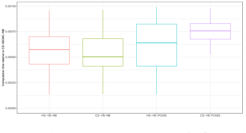
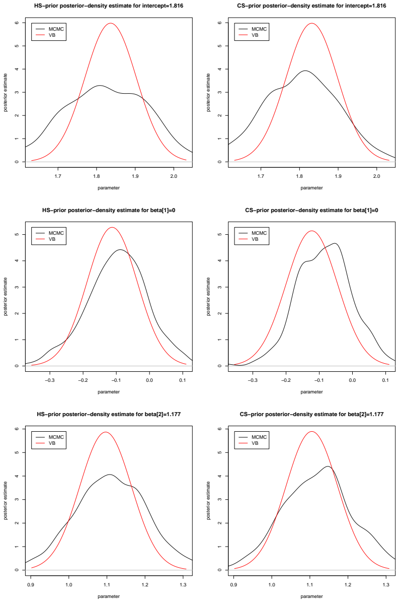
The central claim is that the non-conjugate negative binomial likelihood can be handled inside a mean-field variational Bayes loop by rewriting each count as a Poisson variable with a Gamma-distributed latent rate, and by updating the dispersion parameter through a ratio of special-function integrals denoted H. The resulting closed-form updates for the horseshoe and continuous spike-and-slab priors produce posterior means, variable selections, and predictive distributions close to MCMC benchmarks, with coverage of nominal 95% HPD intervals around 0.79–0.92 under negative binomial data. Under overdispersed data, Poisson-based variational counterparts have coverage between 0.14 and 0.29, which
What carries the argument
The machinery is non-conjugate mean-field variational Bayes: the posterior is approximated as a product of factorized densities, and the regression-coefficient block is forced to be Gaussian, updated with fixed-point equations derived from the non-conjugate VB framework. The negative binomial likelihood is re-expressed as yi|gi ~ Poisson(gi), gi|β ~ Gamma(κ, κ exp(−Xiβ)), which makes the latent gi conditionally conjugate. The dispersion parameter κ has a variational density whose shape is exp{n(κ log κ − log Γ(κ)) − C κ} κ^{1/2}, and its normalizer is an integral called H(p, q, κ, s, t) = ∫ x^p [log(1+κx)]^q [x/Γ(x)]^s exp(−tx) dx. The update for the posterior mean μκ is a ratio of two H-fun
Load-bearing premise
The method assumes the posterior can be approximated as a product of independent factors and that the special H-function formula that normalizes the dispersion parameter's distribution is correct; if the true posterior ties κ and β together strongly, or if that normalizer is off, the updates are biased.
What would settle it
Numerically integrate the kernel exp{n(κ log κ − log Γ(κ)) − C κ} κ^{1/2} over κ and compare the result to the paper's H(−1/2, 0, 1, n, C) expression; a mismatch would bias μκ and all downstream updates. A second, cheaper check: on a small simulated dataset with known coefficients and known overdispersion, compute 95% HPD intervals from the variational posterior and count how often they contain the truth—the paper's own low-dimensional coverage values (0.79–0.92) suggest the intervals are too narrow.
If this is right
- Variational Bayesian sparse negative binomial regression is feasible and fast in high dimensions where MCMC is impractical.
- Users analyzing overdispersed counts can switch from Poisson variational models to negative binomial variational models without giving up computational speed.
- The methods provide full approximate posteriors, enabling HPD intervals and predictive distributions (assessed via CRPS), not just point estimates.
- Among the two priors, the continuous spike-and-slab variant tends to outperform the horseshoe in the high-dimensional case, according to the paper's simulations.
- For data that are actually Poisson, the negative binomial variational methods remain robust, making them a safer default in applied count-data settings.
Where Pith is reading between the lines
- The gap between the reported 79–92% coverage and the nominal 95% suggests that the mean-field factorization or the H-function normalizer in the κ update may be understating posterior uncertainty; a corrected normalizer could close part of that gap.
- With the large computational savings, these methods could make full Bayesian variable selection routine for overdispersed count data with thousands of predictors—settings currently served mainly by penalized likelihood.
- A natural next step is zero-inflated negative binomial regression, where the same auxiliary Gamma representation could handle overdispersion while a separate inflation component handles excess zeros.
- The hard-thresholding step discards the variational inclusion probabilities; replacing it with a threshold based directly on those probabilities might improve variable selection without extra computation.
Editorial analysis
A structured set of objections, weighed in public.
Referee Report
Summary. The paper develops mean-field variational Bayes algorithms for sparse negative binomial regression under horseshoe and continuous spike-and-slab priors (HS-VB-NB and CS-VB-NB). It derives coordinate-ascent updates via the non-conjugate VB framework of Wand et al. (2011), adds a hard-thresholding step for sparse point estimates, and approximates the posterior predictive mass function using a second-order Taylor expansion in the dispersion parameter. Simulations compare the methods with MCMC, penalized likelihood, and Poisson VB competitors in low- and high-dimensional settings; five/six real count datasets are used for predictive evaluation. The abstract and conclusions claim that the negative binomial specification is essential for overdispersed data and is a safer default than Poisson. The paper's own real-data results undermine this headline claim, and there are internal inconsistencies in the HS model derivation.
Significance. If the algorithms were correct and the claims supported, the paper would offer a useful computational tool for high-dimensional negative binomial regression, with speed advantages over MCMC and an explicit variable-selection mechanism. The reported computational savings and the availability of code are genuine strengths. However, the central claim that NB is 'essential' and 'safer' under overdispersion is contradicted by the real-data analysis, and the HS-VB-NB derivation/algorithm does not match the stated model. As presented, the paper's main conclusions are not established; the methodological contribution would need substantial revision and re-evaluation.
major comments (4)
- [Table 4; Abstract; Section 6] The real-data results directly contradict the abstract's claim that NB is 'essential' under overdispersion and 'a safer default. All six benchmark sets are documented as overdispersed in Table 3, yet Poisson VB methods have much lower CRPS on every set (e.g., affairs 0.852 vs 3.968; bike sharing 15.892 vs 218.103; azpro 2.514 vs 10.450) and lower TSRE on five of six sets. The text dismisses this as 'narrower predictive distributions,' but CRPS is a proper scoring rule; consistently lower CRPS indicates better-calibrated predictive distributions, not merely narrower ones. This is a load-bearing contradiction of the paper's main message, and the conclusion repeats the unsupported claim.
- [Section 3, Eq. (13); Algorithm 2; Appendix A] The HS model in Eq. (13) treats the intercept separately with β0|τ0, τ0|a, while βj|Λj,Ξ only for j=1,...,p−1. However, Appendix A's HS derivation uses a joint prior β^T diag(Λ^{-2})β including β0, and Algorithm 2 updates E(Λ^{-1}_j) for j=0,...,p−1 and omits any update for τ0 or a. This means the implemented HS-VB-NB updates are not the variational Bayes updates for the model stated in Eq. (13). The reported HS-VB-NB simulation and real-data results therefore correspond to an unspecified or different model, undermining reproducibility and validity.
- [Table 1; Section 4.1; Section 6] The paper claims uncertainty quantification 'comparable to MCMC benchmarks' (Section 6), but Table 1 shows HS-VB-NB and CS-VB-NB HPD coverage of 0.79–0.92 at nominal 0.95, while the MCMC benchmarks attain 0.94–1.00. The text describes 0.79–0.92 as 'close to the nominal level,' which is not accurate for a 95% interval, especially for the intercept (0.79–0.80). This undercoverage is a known consequence of mean-field VB and should be reported as a limitation, not as comparable uncertainty quantification.
- [Section 3.2; Table 4] The posterior predictive mass function used for CRPS is based on a second-order Taylor expansion of the integrand around μκ, without any validation against an MCMC predictive distribution. Since CRPS in Table 4 is computed from this approximate predictive CDF, the real-data comparison between NB and Poisson methods is not reliable evidence for either method's predictive performance. At minimum, the paper should check this approximation (e.g., on the low-dimensional fishing data where MCMC is available) before drawing conclusions about predictive superiority.
minor comments (4)
- [Section 3 title] Typo: 'negitive' should be 'negative.' Other typos include 'Gammma,' 'Inv-Gammma,' 'derivaties,' and 'disscussed.'
- [Table 3 / Section 5] The text says '5 benchmark real data sets,' but Table 4 reports results for six, and Table 3 lists both azpro and azprocedure with identical rows. Clarify the number of datasets and remove the duplicate.
- [Eq. (16)] The normalization in Eq. (16) is consistent with the Appendix's κ^{-1/2} kernel: H(−1/2,0,1,n,C) is the normalizer and H(1/2,...)/H(−1/2,...) is the mean. The notation is hard to parse due to formatting; a clearer fraction display would help.
- [Section 3 / Eq. (13)] The hyperparameters M_η are set to 0.01 for η=κ, σ^2, λ, ξ, but the model also includes M_{τ0} for the intercept prior in the HS specification; its value is not specified.
Circularity Check
No significant circularity: the VB derivation is self-contained and the self-citations are not load-bearing.
full rationale
The paper's derivation chain proceeds from a stated hierarchical negative binomial model and explicit mean-field factorization to closed-form VB updates via the non-conjugate framework of Wand et al. (2011) and the Poisson-Gamma representation attributed to Luts and Wand (2015). The updates for q(β), q(g), q(κ), and the ELBO are derived in Appendix A from the joint log-density; none of these steps defines a parameter in terms of the quantity it is later used to predict. The μκ expression H(1/2)/H(−1/2) is the expectation under the stated q(κ) kernel, so it is definitional rather than circular. The self-citation to Kharabati et al. (2026) is used only to identify the CS-VB-POISS benchmark and does not supply an unverified load-bearing premise such as a uniqueness theorem. The simulation design does generate data from a negative binomial model, which makes the qualitative finding that NB outperforms Poisson under that DGP unsurprising, but this is a simulation-design/validity concern rather than an equation-level circularity; moreover, the real-data Table 4 actually undercuts the headline 'NB is essential' claim, which further indicates the issue is correctness/overgeneralization, not circular reasoning. Hyperparameter choices (c=0.001, Mη=0.01) and AIC-based thresholding are tuned quantities, but they are evaluated on held-out test sets for TSRE and CRPS, so they are not being relabeled as predictions. Overall, no circular step meeting the required evidentiary standard was found.
Axiom & Free-Parameter Ledger
free parameters (4)
- c (spike scale ratio in CS prior) =
0.001
- M_eta hyperparameters =
0.01 for κ, σ², λ, ξ
- alpha_1, alpha_2 =
1, 1
- hard-threshold tau_hat =
selected by AIC over a grid
axioms (5)
- domain assumption Mean-field factorization q(θ) = ∏ q(θ_j)
- standard math Gamma-Poisson mixture representation of the negative binomial
- domain assumption Wand et al. non-conjugate VB fixed-point equations apply
- domain assumption AIC is an efficient proxy for leave-one-out cross-validation for threshold selection
- ad hoc to paper Second-order Taylor expansion around μ_κ approximates the predictive integral
read the original abstract
Count data with overdispersion and high-dimensional predictors pose significant challenges in modern applications. While negative binomial regression offers a flexible modeling framework, existing Bayesian approaches rely on computationally expensive MCMC methods that become impractical in high-dimensional settings. This paper develops a variational Bayesian framework for sparse negative binomial regression using horseshoe and continuous spike-and-slab priors. Our proposed methods achieve estimation accuracy and variable selection performance comparable to MCMC benchmarks while offering substantial computational savings over MCMC. Extensive simulations demonstrate that the negative binomial specification is essential for overdispersed data, as Poisson-based approaches exhibit substantial performance degradation under overdispersion. Conversely, our methods remain robust when the data are Poisson, making them a safer default choice. Applications to real benchmark datasets further confirm the practical utility of our approach.
Figures




Reference graph
Works this paper leans on
-
[1]
Ahmed, S. E. (2014). Estimation Strategies in Poisson Regression Models. Penalty, Shrinkage, and Pretest Strategies: Variable Selection and Estimation, 101-115
2014
-
[2]
Algamal, Z. Y. (2015). Penalized Poisson regression model using adaptive modified elastic net penalty. Electronic Journal of Applied Statistical Analysis, 8(2), 236-245
2015
-
[3]
M., Collins, M
Bailey, D. M., Collins, M. A., Gordon, J. D., Zuur, A. F., & Priede, I. G. (2009). Long-term changes in deep-water fish populations in the northeast Atlantic: a deeper reaching effect of fisheries? Proceedings of the Royal Society B: Biological Sciences, 276(1664), 1965-1969
2009
-
[4]
M., Kucukelbir, A., & McAuliffe, J
Blei, D. M., Kucukelbir, A., & McAuliffe, J. D. (2017). Variational inference: A review for statisticians. Journal of the American Statistical Association, 112(518), 859-877
2017
-
[5]
M., Polson, N
Carvalho, C. M., Polson, N. G., & Scott, J. G. (2009). Handling sparsity via the horseshoe. Journal of Machine Learning Research W&CP, 5, 73-80
2009
-
[6]
H., & Ibrahim, J
Chen, M. H., & Ibrahim, J. G. (2000). Bayesian predictive inference for time series count data. Biometrics, 56(3), 678-685
2000
-
[7]
L., & Morris, C
Christiansen, C. L., & Morris, C. N. (1997). Hierarchical Poisson regression modeling. Journal of the American Statistical Association, 92(438), 618-632
1997
-
[8]
G., & Aiken, L
Coxe, S., West, S. G., & Aiken, L. S. (2009). The analysis of count data: A gentle introduction to Poisson regression and its alternatives. Journal of Personality Assessment, 91(2), 121-136
2009
-
[9]
Datta, J., & Dunson, D. B. (2016). Bayesian inference on quasi-sparse count data. Biometrika, 103(4), 971-983
2016
-
[10]
L., & Johnstone, I
Donoho, D. L., & Johnstone, I. M. (1994). Ideal spatial adaptation by wavelet shrinkage. Biometrika, 81(3), 425-455
1994
-
[11]
El-Sayyad, G. M. (1973). Bayesian and classical analysis of Poisson regression. Journal of the Royal Statistical Society: Series B (Methodological), 35(3), 445-451
1973
-
[12]
Fair, R. C. (1978). A theory of extramarital affairs. Journal of political economy, 86(1), 45-61
1978
-
[13]
Fan, J., & Li, R. (2001). Variable selection via nonconcave penalized likelihood and its oracle properties. Journal of the American Statistical Association, 96(456), 1348-1360
2001
-
[14]
Fu, S. (2015). A hierarchical Bayesian approach to negative binomial regression. Methods and Applications of Analysis, 22(4), 409-428
2015
-
[15]
Fu, S. (2016). Hierarchical Bayesian LASSO for a negative binomial regression. Journal of Statistical Computation and Simulation, 86(11), 2182-2203
2016
-
[16]
I., & McCulloch, R
George, E. I., & McCulloch, R. E. (1993). Variable selection via Gibbs sampling. Journal of the American Statistical Association, 88(423), 881-889
1993
-
[17]
I., & McCulloch, R
George, E. I., & McCulloch, R. E. (1997). Approaches for Bayesian variable selection. Statistica Sinica, 7(2),339-373
1997
-
[18]
Greene, W. H. (2003). Econometric analysis. Pearson Education India
2003
-
[19]
Hilbe, J. M. (2011). Negative binomial regression. Cambridge University Press
2011
-
[20]
Ishwaran, H., & Rao, J. S. (2003). Detecting differentially expressed genes in microarrays using Bayesian model selection. Journal of the American Statistical Association, 98(462), 438-455
2003
-
[21]
Ishwaran, H., & Rao, J. S. (2005). Spike and slab variable selection: frequentist and Bayesian strategies. Annals of Statistics, 33(2), 730-773
2005
-
[22]
Jia, J., Xie, F., & Xu, L. (2019). Sparse Poisson regression with penalized weighted score function. Electronic Journal of Statistics, 13(2), 2898-2920
2019
-
[23]
Kharabati, M., Amini, M., & Arashi, M. (2026). Variational inference for sparse Poisson regression. Computational Statistics, 41(3), 67
2026
-
[24]
G., & Albert, P
Kim, S., Chen, Z., Zhang, Z., Simons-Morton, B. G., & Albert, P. S. (2013). Bayesian hierarchical Poisson regression models: an application to a driving study with kinematic events. Journal of the American Statistical Association, 108(502), 494-503
2013
-
[25]
Luts, J., & Wand, M. P. (2015). Variational inference for count response semiparametric regression. Bayesian Analysis, 10(4), 991-1023
2015
-
[26]
Mitchell, T., & Beauchamp, J. (1988). Bayesian variable selection in linear regression. Journal of the American Statistical Association, 83(404), 1023-1032
1988
-
[27]
Murru, V., & Wand, M. P. (2025). Variational Inference for Count Response Semiparametric Regression: A Convex Solution. arXiv preprint arXiv:2510.12356
arXiv 2025
-
[28]
T., You, C., & Müller, S
Ormerod, J. T., You, C., & Müller, S. (2017). A variational Bayes approach to variable selection. Electronic Journal of Statistics, 11(2), 3549-3594
2017
-
[29]
G., Scott, J
Polson, N. G., Scott, J. G., & Windle, J. (2014). The Bayesian Bridge. Journal of the Royal Statistical Society Series B: Statistical Methodology, 76(4), 713-733
2014
-
[30]
Ray, K., & Szabó, B. (2022). Variational Bayes for high-dimensional linear regression with sparse priors. Journal of the American Statistical Association, 117(539), 1270-1281
2022
-
[31]
Soussen, C., Idier, J., Brie, D., & Duan, J. (2011). From Bernoulli-Gaussian deconvolution to sparse signal restoration. IEEE Transactions on Signal Processing, 59(10), 4572-4584
2011
-
[32]
Tibshirani, R. (1996). Regression shrinkage and selection via the lasso. Journal of the Royal Statistical Society Series B: Statistical Methodology, 58(1), 267-288
1996
-
[33]
P., Ormerod, J
Wand, M. P., Ormerod, J. T., Padoan, S. A., & Frühwirth, R. (2011). Mean field variational Bayes for elaborate distributions. Bayesian Analysis, 6(4), 847-900
2011
-
[34]
Zeileis, A., Kleiber, C., and Jackman, S. (2008). Regression models for count data in R. Journal of Statistical Software, 27(8):1--25
2008
-
[35]
Zhang, H., & Jia, J. (2022). Elastic-net regularized high-dimensional negative binomial regression. Statistica Sinica, 32(1), 181-207
2022
-
[36]
F., Hilbe, J
Zuur, A. F., Hilbe, J. M., & Leno, E. N. (2013). A beginner's guide to GLM and GLMM with R: A frequentist and Bayesian perspective for ecologists, 270 p Newburgh. UK: Highland Statistics Ltd
2013
discussion (0)
Sign in with ORCID, Apple, or X to comment. Anyone can read and Pith papers without signing in.