REVIEW 2 major objections 4 minor 24 references
Quantum logistic map considered as discrete-time Heisenberg equation
T0 review · 2 major / 4 minor · reviewed 2026-08-01 · deepseek-v4-flash
Pith's one-line read The paper promotes the scalar logistic map to a multiplication operator on L²([0,1]) and proves exact fixed matrix-element limits for three parameter regimes, with the r=4 case giving exponential approach to δ/2.
desk verdict Correct exact fixed-element asymptotics for the logistic multiplication operator in three regimes, with honest scoping; the numerical section is modest and a typo in the exploratory recursion needs fixing. read the letter →
The pith
A machine-rendered reading of the paper's core claim, the machinery that carries it, and where it could break.
The reading
What carries the argument
The machinery is the promotion of scalar logistic iterates to multiplication operators by functional calculus, X_n = p_n(M_u;r), and evaluation of matrix elements ⟨φ_k, X_n φ_l⟩ in the normalized shifted-Legendre basis. Three analytic tools carry the proofs: dominated convergence after almost-everywhere convergence to the attracting fixed point at r=5/2; an exact phase-basin decomposition of the attracting two-cycle—the countable exceptional set E, intervals I_j and I_j^*, phases (a,b) and (b,a)—at r=16/5; and the conjugacy u=sin²θ with p_n(u;4)=sin²(2ⁿθ), together with Chebyshev polynomial product identities, at r=4. The Chebyshev-moment representation is the identity that converts the osci
What would settle it
Compute x_00(20;4) from the paper's exact Chebyshev-moment formula (26) with N=2²⁰; Theorem 2 asserts |x_00(20;4) − 1/2| ≤ 2/(3(2²⁰)²). A violation of that bound would refute the claimed O(4⁻ⁿ) estimate. For r=16/5, approximate x_00(n;16/5) by adaptive quadrature for even and odd n up to a few hundred; the even and odd subsequences should converge to a + (b−a)∫_{S_ba}φ_0² du and b − (b−a)∫_{S_ba}φ_0² du, respectively, and their sum should approach (21/16).
Extended reading notes
Core claim
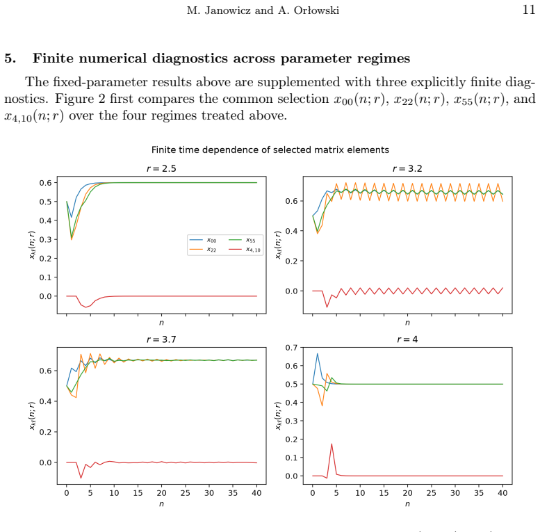
The central claim is that the multiplication-operator iterates X_n = p_n(M_u;r) on L²([0,1]) have fixed shifted-Legendre matrix elements x_kl(n;r) whose limits are exactly known in three regimes. Proposition 1 states x_kl(n;5/2) → (3/5)δ_kl. Theorem 1 gives phase-resolved subsequential limits at r=16/5, with even and odd limits expressed as aδ_kl + (b−a)∫_{S_ba}φ_kφ_l du and bδ_kl − (b−a)∫_{S_ba}φ_kφ_l du, summing to (21/16)δ_kl. Theorem 2 provides an exact finite Chebyshev-moment representation at r=4 yielding x_kl(n;4) = δ_kl/2 + O_kl(4⁻ⁿ). The paper emphasizes these statements concern fixed basis indices and do not imply operator-norm convergence, and they are distinct from the finite-res
Load-bearing premise
For the analytic theorems, the load-bearing premise is that the scalar logistic iterates converge pointwise almost everywhere in each regime (to 3/5 at r=5/2, to the two-cycle phases away from a countable set at r=16/5, and to the conjugacy picture at r=4), so dominated convergence applies to the fixed basis elements; for the chaotic section, the premise is that the finite equal-stratum quadrature with the stated offsets and horizons is representative enough for the stabilize
Editorial extensions
If this is right
- If the central claims are correct, fixed diagonal matrix elements of the multiplication-operator iterates equilibrate to scalar multiples of the identity in the regular regimes, so the operator picture inherits the scalar dynamics for fixed indices.
- At r=16/5 the phase-basin structure becomes visible in operator matrix elements through integrals over S_ba, meaning the two-cycle's basin geometry has a direct operator-level signature.
- At r=4 the fixed elements approach δ/2 exponentially fast, with the explicit bound |x_kl(n;4) − δ_kl/2| ≤ 2 S_kl A_kl / (3(N−d)²), N=2ⁿ, for N>d.
- Because the results are fixed-element and not operator-norm, finite-dimensional truncations of the nonlinear recursion cannot be assumed equivalent to compressing the functional-calculus result; the paper states this inequivalence explicitly.
- The sum rule x_even_kl + x_odd_kl = (21/16)δ_kl at r=16/5 is an exact fixed-element identity that a numerical simulation can verify directly.
Reading between the lines
- The paper leaves implicit that the r=4 proof, relying only on angle doubling and Chebyshev moments, should extend to any map conjugate to angle doubling; a testable extension is the same fixed-element O(4⁻ⁿ) rate for the tent map's conjugate form.
- A direct extension is to compute the phase-basin integrals ∫_{S_ba} φ_k φ_l du in closed form for low k,l, using the explicit interval endpoints c_j; this would turn Theorem 1 into fully explicit numerical constants.
- For the chaotic regime r=37/10, the paper's stabilization of finite Cesàro means suggests a testable diagnostic: run the same deterministic quadrature with larger horizons and finer strata; if the late-window means continue to stabilize, that supports—but never proves—an invariant-measure interpretation.
- The separate finite-matrix recursion X_{k+1}=R X_k(I−X_k)R† is left exploratory; a natural editorial follow-up is to seek sufficient conditions on R preserving 0≤X_k≤I, which the paper names as future work but does not attempt.
Editorial analysis
A structured set of objections, weighed in public.
Referee Report
Summary. The manuscript represents the scalar logistic iterates p_n(·;r) as multiplication operators X_n = p_n(M_u) on L^2([0,1]) and studies fixed matrix elements in the normalized shifted-Legendre basis. Three parameter regimes are treated analytically: r=5/2 (Prop. 1, Eq. (10): every fixed matrix element converges to (3/5)δ_kl), r=16/5 (Thm. 1, Eqs. (17)–(19): phase-resolved even and odd subsequential limits arising from an exact basin decomposition of the period-two attractor), and r=4 (Thm. 2, Eqs. (26)–(29): an exact Chebyshev-moment representation giving x_kl(n;4)=δ_kl/2+O_kl(4^{-n})). The remaining material is explicitly finite and numerical: a controlled refinement study at r=37/10, finite-time diagnostics (matrix-element time series, bifurcation-style plot, intensity moments, scalar OTOC-type Gram matrices), and a separate finite-dimensional recursion X_{k+1}=R X_k(I-X_k)R^†. The paper repeatedly disclaims operator-norm convergence, invariant-measure or ergodic conclusions, and asymptotic claims in the chaotic regime.
Significance. If the analytical statements are taken with the correction noted below, the paper provides correct and carefully delimited results. The proofs of Prop. 1 and Thm. 1 are standard dominated-convergence and basin-decomposition arguments; Thm. 2 gives an exact fixed-element representation at r=4 with a clean O(4^{-n}) bound. A notable strength is the explicit separation of proved fixed-element statements from finite numerical observations, and the absence of fitted parameters or assumed limit values in the analytical claims. The novelty is modest—the multiplication-operator interpretation is largely formal—but the paper is a solid, honest contribution suitable for a mathematical physics journal once the typographical issue in Eq. (26) is fixed.
major comments (2)
- [4.2, Eq. (26)] The displayed formula has a sign error in the numerator. From the product identity T_m(y)T_N(y) = (T_{m+N}(y)+T_{|m-N|}(y))/2, the integrated bracket should be μ_m − (μ_{m+N}+μ_{|m-N|})/2, i.e. (2μ_m − μ_{m+N} − μ_{|m-N|})/2, not (μ_m − μ_{m+N}+μ_{|m-N|})/2. With the printed sign, the case k=l=0 gives x_00(n;4)=1/4, contradicting direct integration (which gives 1/2 − μ_N/4). The subsequent bound in Eq. (28) is consistent with the corrected sign, so the final O(4^{-n}) claim is unaffected, but Eq. (26) must be corrected before publication.
- [6, Eq. (41)] The definition d_C(n)=2e^{γ_C n}e^{-γ_C n} simplifies identically to the constant 2. The text and Fig. 7 describe three distinct amplitude profiles, and the pairwise-distance values D_AC, D_BC are interpreted as comparisons of different profiles. As written, profile C is constant, so these comparisons do not probe an exponentially varying profile. If an exponentially decaying or otherwise nontrivial profile was intended, the formula should be corrected (e.g. 2e^{-γ_C n} or 2(1−e^{-γ_C n})); if the constant profile is intentional, the wording should state so explicitly.
minor comments (4)
- [3.2, proof of Thm. 1] The statement 'On [c_1,q], the only critical point of g is 1/2' is used to identify g([c_1,q])=[64/125,q]. This is true, but it requires checking that f(f(u))=1/2 has no solution in [c_1,q] besides u=1/2; the two roots of (16/5)u(1−u)=1/2 are approximately 0.194 and 0.806, both outside the interval. Please add a sentence with this verification.
- [4.1, Eq. (21)] The claim that the finite Cesàro and late-window means are 'substantially more stable' under the described refinements is qualitative. Since the section explicitly disclaims asymptotic conclusions, this is not a correctness defect, but a compact table of representative values across N and s would make the observation more reproducible and less dependent on figure inspection.
- [Title and §2.1] The title's 'discrete-time Heisenberg equation' may mislead readers, since the update is not unitary and is not the standard Heisenberg equation. Section 2.1 already clarifies this, but the title remains suggestive. Consider a more neutral title such as 'Multiplication-operator dynamics of the logistic map and fixed matrix elements'.
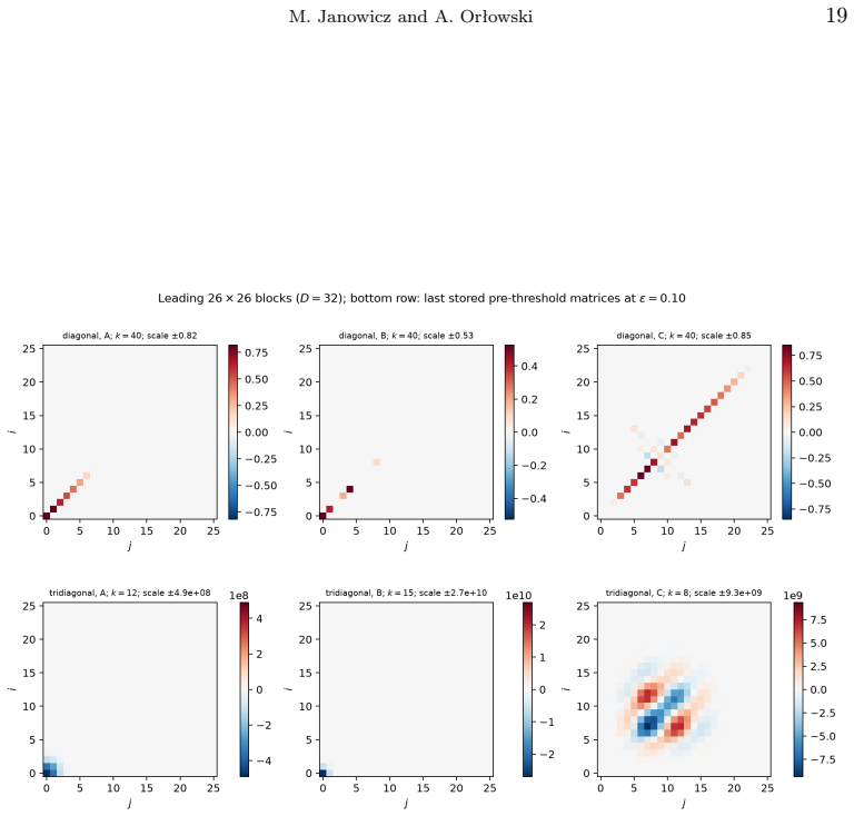
- [6.1, Fig. 8 caption] The caption lists the last stored steps as k=12,15,8, which matches the order A, B, C, but the text states profile C crosses the threshold at k=9 (last stored k=8), profile A at k=13 (last stored k=12), and profile B at k=16 (last stored k=15). Reordering or an explicit cross-reference would avoid a quick misreading.
Circularity Check
No significant circularity: analytical limits are derived from scalar logistic dynamics and proved identities; numerical sections are explicitly finite and make no asymptotic claims.
full rationale
The paper's derivations are self-contained reductions of analytic statements to standard facts about the logistic map. Prop. 1 uses the attracting fixed point 3/5 and dominated convergence; the limit is not inserted as an ansatz. Theorem 1 derives the phase-basin decomposition via Eq. (15) and the inverse branch (12), then obtains the subsequential limits by dominated convergence; the basin set S_ba is a consequence of the interval dynamics, not a fitted input. Theorem 2 follows from the exact conjugacy p_n(u;4)=sin^2(2^n theta), the substitution u=sin^2 theta, t=2 theta, y=cos t, and the finite Chebyshev product identity (25); the O(4^{-n}) estimate is a bound on the oscillatory part. No parameter is fitted to the quantities being predicted, and the fixed matrix elements are evaluated directly from the defined multiplication-operator sequence. There are no load-bearing self-citations: the cited references [10]-[24] provide background or external context only, not the uniqueness or existence of the limits. The r=37/10 section is explicitly finite numerical diagnostics and repeatedly disclaims asymptotic, invariant-measure, and operator-norm conclusions (e.g. Section 4.1: 'They do not establish convergence...'), so it cannot be circular. The exploratory matrix recursion in Section 6 is labelled as separate and finite-time, with no general theorem claimed. Therefore no circularity step is present.
Assumptions & free parameters
free parameters (6)
- γ_A =
0.10
- γ_B =
0.08
- ω =
π/4
- γ_C =
0.12 (canceled in Eq. 41 as written)
- ε =
0.10
- D =
32
assumptions (5)
- standard math Dominated convergence theorem; orthonormality of the shifted-Legendre basis.
- standard math Chebyshev product-to-sum identity and Chebyshev integral formula.
- domain assumption Logistic-at-4 conjugacy p_n(u;4)=sin^2(2^n θ) for u=sin^2 θ.
- domain assumption Endpoint/preimage sets are exceptional: at r=5/2 the bad set is {0,1}; at r=16/5 the bad set E is countable.
- domain assumption Forward invariance 0≤p_n(u;r)≤1 for r∈(0,4], u∈[0,1].
Cite this review
Pith. "Pith review of Quantum logistic map considered as discrete-time Heisenberg equation." pith.science (2026). https://pith.science/paper/5GOMMHJS
@misc{pith2026260719159,
  author       = {Pith},
  title        = {Pith review of: Quantum logistic map considered as discrete-time Heisenberg equation},
  year         = {2026},
  howpublished = {\url{https://pith.science/paper/5GOMMHJS}},
  note         = {Machine review of arXiv:2607.19159}
}
abstract
We represent scalar logistic iterates as multiplication operators on $L^2([0,1])$ and study their fixed matrix elements in the normalized shifted-Legendre basis. Three parameter regimes permit analytical control. At $r=5/2$, every fixed matrix element converges to $3\delta_{kl}/5$, where $\delta_{kl}$ is the Kronecker delta. At $r=16/5$, the attracting period-two orbit yields phase-resolved limits for the even and odd subsequences. At $r=4$, an exact Chebyshev-moment representation gives an $O(4^{-n})$ approach of every fixed matrix element at iteration $n$ to $\delta_{kl}/2$. The case $r=37/10$ is treated only by a controlled finite numerical refinement study. Complementary finite diagnostics comprise matrix-element time dependence, a bifurcation-style plot, a time-averaged mean intensity, a normalized second-order intensity moment, and normalized scalar OTOC-type commutator correlation matrices. We also examine the separate finite-dimensional recursion $X_{k+1}=R X_k(I-X_k)R^\dagger$, with fixed matrix $R$, using diagonal and tridiagonal amplitude profiles. These operator-valued calculations are exploratory finite-time numerics. The analytical statements concern fixed matrix elements for the specified basis indices; they are distinct from the finite-resolution observations and do not imply operator-norm convergence. A regularized phase-space lift is included as a controlled visualization.
Figures


Figures from the paper (5 more)


Reference graph
Works this paper leans on
-
[1]
Birkhäuser, Boston, 1980
Pierre Collet and Jean-Pierre Eckmann.Iterated Maps on the Interval as Dynamical Sys- tems. Birkhäuser, Boston, 1980
1980
-
[2]
Adam Hilger, Bristol, 2 edition, 1989
Predrag Cvitanović, editor.Universality in Chaos. Adam Hilger, Bristol, 2 edition, 1989
1989
-
[3]
Devaney.An Introduction to Chaotic Dynamical Systems
Robert L. Devaney.An Introduction to Chaotic Dynamical Systems. Addison-Wesley, Reading, MA, 2 edition, 1989
1989
-
[4]
Eckmann and D
J.-P. Eckmann and D. Ruelle. Ergodic theory of chaos and strange attractors.Reviews of Modern Physics, 57(3):617–656, 1985
1985
-
[5]
Feigenbaum
Mitchell J. Feigenbaum. Quantitative universality for a class of nonlinear transformations. Journal of Statistical Physics, 19(1):25–52, 1978
1978
-
[6]
Cambridge Univer- sity Press, Cambridge, 2 edition, 2004
Holger Kantz and Thomas Schreiber.Nonlinear Time Series Analysis. Cambridge Univer- sity Press, Cambridge, 2 edition, 2004
2004
-
[7]
Robert M. May. Simple mathematical models with very complicated dynamics.Nature, 261(5560):459–467, 1976
1976
-
[8]
Cambridge University Press, Cambridge, 2 edition, 2002
Edward Ott.Chaos in Dynamical Systems. Cambridge University Press, Cambridge, 2 edition, 2002
2002
Show all 24 references
-
[9]
Strogatz.Nonlinear Dynamics and Chaos
Steven H. Strogatz.Nonlinear Dynamics and Chaos. Westview Press, Boulder, CO, 2 edition, 2015
2015
-
[10]
Matrix logistic map: fractal spectral distributions and transfer of chaos.arXiv preprint, 2025
Łukasz Pawela and Karol Życzkowski. Matrix logistic map: fractal spectral distributions and transfer of chaos.arXiv preprint, 2025
2025
-
[11]
M. E. Goggin, B. Sundaram, and P. W. Milonni. Quantum logistic map.Physical Review A, 41(10):5705–5708, 1990
1990
-
[12]
Michael V. Berry. Regular and irregular semiclassical wavefunctions.Journal of Physics A: Mathematical and General, 10(12):2083–2091, 1977
-
[13]
Gutzwiller.Chaos in Classical and Quantum Mechanics
Martin C. Gutzwiller.Chaos in Classical and Quantum Mechanics. Springer-Verlag, New York, 1990
1990
-
[14]
Springer, Berlin Heidelberg, 3 edition, 2010
Fritz Haake.Quantum Signatures of Chaos. Springer, Berlin Heidelberg, 3 edition, 2010. M. Janowicz and A. Orłowski22
2010
-
[15]
World Scientific, Singapore, 2000
Viviane Baladi.Positive Transfer Operators and Decay of Correlations. World Scientific, Singapore, 2000
2000
-
[16]
Andrzej Lasota and James A. Yorke. On the existence of invariant measures for piecewise monotonic transformations.Transactions of the American Mathematical Society, 186:481– 488, 1973
1973
-
[17]
Resonances of chaotic dynamical systems.Physical Review Letters, 56(5):405–407, 1986
David Ruelle. Resonances of chaotic dynamical systems.Physical Review Letters, 56(5):405–407, 1986
1986
-
[18]
Ulam.A Collection of Mathematical Problems
Stanislaw M. Ulam.A Collection of Mathematical Problems. Interscience Publishers, New York, 1960
1960
-
[19]
A. I. Larkin and Yu. N. Ovchinnikov. Quasiclassical method in the theory of superconduc- tivity.Soviet Physics JETP, 28(6):1200–1205, 1969
1969
-
[20]
Shenker, and Douglas Stanford
Juan Maldacena, Stephen H. Shenker, and Douglas Stanford. A bound on chaos.Journal of High Energy Physics, 2016(8):106, 2016
2016
-
[21]
Rozenbaum, Sriram Ganeshan, and Victor Galitski
Efim B. Rozenbaum, Sriram Ganeshan, and Victor Galitski. Lyapunov exponent and out-of-time-ordered correlator’s growth rate in a chaotic system.Physical Review Letters, 118(8):086801, 2017
2017
-
[22]
Shenker and Douglas Stanford
Stephen H. Shenker and Douglas Stanford. Black holes and the butterfly effect.Journal of High Energy Physics, 2014(3):67, 2014
2014
-
[23]
Unscrambling the physics of out-of-time-order correlators.Nature Physics, 14(10):988–990, 2018
Brian Swingle. Unscrambling the physics of out-of-time-order correlators.Nature Physics, 14(10):988–990, 2018
2018
-
[24]
Rényi extrapolation of Shannon entropy.Open Systems & Information Dynamics, 10(3):297–310, 2003
Karol Życzkowski. Rényi extrapolation of Shannon entropy.Open Systems & Information Dynamics, 10(3):297–310, 2003
2003
Reviewed August 1, 2026 · model on record in the stance chip above.
Discussion (0). Continue with ORCID to comment.