REVIEW 3 major objections 4 minor 70 references
Optical polarization in blazar 1ES 1959+650 tracks brightness before a flare, anti-tracks after, decouples during it; paper attributes flip to jet viewing angle.
Reviewed by Pith at T0; open to challenge. T0 means a machine referee read the full paper against a public rubric. the ladder, T0–T4 →
T0 review · deepseek-v4-flash
2026-08-01 11:26 UTC pith:2SPXFRIA
load-bearing objection Solid new epoch-dependent PD–flux correlation for 1ES 1959+650; the geometry explanation is a fit, not a tested prediction. the 3 major comments →
Peculiar Behavior of Optical Polarization in Blazar 1ES 1959+650: Role of Jet Magnetic Field and Geometry
The pith
A machine-rendered reading of the paper's core claim, the machinery that carries it, and where it could break.
Core claim
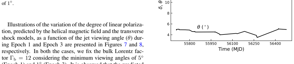
The paper reports that in 1ES 1959+650 the degree of optical linear polarization is strongly positively correlated with V- and R-band fluxes before a major flare, strongly anti-correlated after it, and essentially uncorrelated during the flare itself. It argues that the pre- and post-flare behavior is geometric: observed flux variability is Doppler-factor variability from modest jet viewing-angle changes, and the accompanying polarization response matches a helical magnetic field or a transverse shock in a jet with Gamma_b = 12. The flare epoch is explained by a turbulent multi-zone emission model in which polarization from many misaligned cells partially cancels. The paper thus presents a s
What carries the argument
The central machinery is the assumption that all optical flux variability is Doppler variability: delta = delta_max (F/F_max)^(1/(2+alpha)) converts the measured light curve into a time series of viewing angle theta for fixed bulk Lorentz factor Gamma_b = 12. Two polarization formulae are used: the helical-field expression P_hel = P_max sin^2(theta'), and the transverse-shock expression P_sw proportional to [(alpha+1)/(alpha+5/3)] (1-eta^-2) sin^2(theta') / [2-(1-eta^-2) sin^2(theta')], with theta' the aberrated viewing angle and eta the shock compression. The sign of the correlation between flux and polarization is set by which branch of the polarization-theta curve the relevant theta range
Load-bearing premise
The argument stands on the premise that every optical flux change reflects a Doppler-factor change, i.e., the intrinsic synchrotron power of the emitting region is constant during the pre- and post-flare epochs; if particle injection or magnetic-field strength varies on the same timescales, the inferred viewing angles and the conclusions collapse.
What would settle it
Measure the optical spectral index simultaneously with the V-band flux across the pre- and post-flare epochs; if the spectral index changes systematically with flux, the flux variations cannot be purely geometric Doppler changes, and the inferred viewing-angle series is invalid. Alternatively, a single-zone model with time-varying magnetic field or electron injection that reproduces the same polarization-flux correlations would falsify the uniqueness of the geometric explanation.
If this is right
- If the geometric explanation is right, the optical emission region's viewing angle swung between roughly 5 and 14 degrees before the flare and between 1 and 4 degrees after it, with no change in intrinsic jet power.
- The inferred viewing-angle series can be checked against radio jet kinematics, such as apparent superluminal motion or core-shift measurements, providing an independent test.
- The near-zero polarization-flux correlation during the flare, combined with small polarization-angle changes, supports a turbulent multi-zone origin for the flare.
- Applying the same analysis to other blazars with decade-long polarimetric monitoring would show whether such correlation sign flips are common and viewing-angle driven.
Where Pith is reading between the lines
- The geometric model predicts systematic polarization-angle rotations tied to the inferred viewing-angle swings; the paper reports only modest PA changes, so a quantitative PA comparison would be a sharper test.
- The framework assumes the intrinsic synchrotron luminosity is constant; simultaneous X-ray/TeV light curves during the same epochs could reveal whether the flux variability is truly purely geometric.
- Extending the same decomposition to simulated light curves with known intrinsic particle injection would clarify how easily non-geometric variability could mimic the observed sign flip.
Editorial analysis
A structured set of objections, weighed in public.
Referee Report
Summary. This paper analyzes ~10 years of SPOL/Steward Observatory photopolarimetry of the blazar 1ES 1959+650. It divides the light curve into an optical flaring epoch (MJD 55650–56500, Epoch 2) and two quiescent epochs before and after (Epoch 1: MJD 55000–55500; Epoch 3: MJD 57500–58000). The authors report strong positive correlations between the degree of linear polarization (PD) and V/R-band flux in Epoch 1 (Pearson r ≈ 0.91, Spearman ρ ≈ 0.83, p < 1e-3), strong anti-correlations in Epoch 3 (r ≈ -0.84, ρ ≈ -0.84, p < 1e-3), and no significant correlation in Epoch 2. They interpret these patterns using a helical magnetic field model and a transverse shock model under the assumption that all optical flux variability is caused by changing jet viewing angle (Eq. 4). Inferred viewing-angle ranges are 5°–14° for Epoch 1 and 1°–4° for Epoch 3, with Γ_b = 12. The flare epoch is attributed to turbulent multi-zone emission (TEMZ). The paper concludes that the long-term optical variability can be "purely attributed to time-dependent orientations of the emission region."
Significance. The observational correlation analysis is a strength: the Pearson and Spearman tests, and the ZDCF, consistently support the sign reversal between Epochs 1 and 3, and the SPOL data are public. If the geometric interpretation were independently validated, the paper would add an interesting HBL case where modest jet-orientation changes could explain the sign of the PD–flux correlation. However, the modeling portion is not yet at the same standard. The load-bearing assumption that all flux changes are Doppler-induced is untested, and the helical-field/shock comparison uses per-epoch fitted parameters (P_max, η) and viewing-angle intervals chosen after the fact. The claim that variability can be "purely attributed" to geometry is therefore not supported by the evidence presented. The paper would be suitable after a substantial revision that turns the model comparison into a quantitative, falsifiable test.
major comments (3)
- [Section III.B, Eq. (4)] The entire geometric interpretation rests on Eq. (4), δ = δ_max (F/F_max)^(1/(2+α)), which assumes constant intrinsic synchrotron power and that F_max corresponds to the maximum Doppler factor. But the global F_max occurs in Epoch 2, which the paper itself attributes to turbulent multi-zone intrinsic emission; using that value as the normalization contaminates the derived δ(t) and θ(t) for Epochs 1 and 3. Moreover, Section III.A notes X-ray and TeV flares during Epoch 3 without an optical flare, showing that non-geometric activity is present. The inferred θ ranges (5°–14°, 1°–4°) and the subsequent model comparisons are therefore not established. Please test this assumption (e.g., constancy of spectral index, V/R color, or multi-band ratios) or restrict Eq. (4) to an epoch where the geometric hypothesis is independently supported.
- [Section III.B, Eqs. (5)–(8), Figs. 5–8] The model comparison is largely circular. P_max is set separately for Epochs 1 and 3 (8.5% and 5%), η is set separately (1.128 and 1.070), and the θ intervals are chosen so that Epoch 1 lies on the descending branch of P(θ) and Epoch 3 on the ascending branch. Since the Doppler factor decreases monotonically with θ in this range, the sign of the predicted PD–flux correlation is imposed by selecting which branch of P(θ) is used. No fit statistic, parameter uncertainty, or model-selection criterion is provided. A quantitative fit with uncertainties, and ideally a prediction for the correlation sign from un-fitted data, is needed before "satisfactorily explained" is justified.
- [Section III.A and Section III.B, Epoch 2] The paper uses a geometric, Doppler-only interpretation for Epochs 1 and 3 but attributes the Epoch 2 optical flare to intrinsic turbulent multi-zone emission. These two mechanisms are not reconciled: if the same optical data contain an intrinsically driven flare, then Eq. (4) is not a valid global inversion. The paper needs an explicit criterion for when the geometric mechanism dominates and when the intrinsic mechanism dominates, or it must restrict the geometric model to epochs where intrinsic variability can be excluded. Without this, the internal consistency of the proposed scenario is questionable.
minor comments (4)
- [Section III.A, Table III] The text describing the U–I Stokes correlations contradicts Table III. The text says Epoch 1 shows a strong anti-correlation and Epoch 3 a positive correlation, but Table III gives U–I Spearman coefficients of -0.870 (Epoch 1) and -0.813 (Epoch 3), i.e., both negative. The text also calls the Epoch 2 U–I correlation "very weak positive," while the table lists -0.108. Please correct the text or the table.
- [Section III.B, paragraph after Eq. (7)] There is a typo: "anti-correlations (Epoch 2)" should read "anti-correlation (Epoch 3)" for the PD–flux relation; Epoch 2 shows no significant correlation.
- [Figures 5 and 6 captions] The captions state that the green shaded region represents the "full range of model uncertainty (Equation 5)", but no uncertainty is defined or propagated. Please specify what uncertainties (measurement, parameter, or model) are included in the shaded band.
- [Section III.B, Eq. (7)] The shock model uses α from optical photometric measurements, but the α values and their uncertainties are not given in this paper. Please report them, since P_sw depends sensitively on α.
Circularity Check
Helical/shock 'predictions' of PD–flux correlation are fitted via P_max, η, and per-epoch θ_min; flux-to-θ mapping makes the geometric explanation self-definitional.
specific steps
-
fitted input called prediction
[Section III.B, Eq. (5) and Figs. 5-6 (paragraph after Eq. 5)]
"The model predictions are found to be broadly consistent with the measurements during Epoch 1 and Epoch 3 withP max ∼8.5%and 5%, respectively (Figure 1). ... It is evident that the observed variations in the degree of polarization restrict the viewing angle between5◦ and14◦ during Epoch 1. However, the viewing angle lies in the range1◦ −4◦ during Epoch 3."
P_max is a free normalization chosen so that the PD amplitude from Eq. (5) matches the observed PD for the θ(t) obtained from Eq. (4). The sign of the PD–flux correlation is then set by the arbitrarily chosen per-epoch minimum viewing angle (5° for Epoch 1, 1° for Epoch 3), which places the θ interval on the descending or ascending side of the P(θ) peak at ≈5°. The 'predicted' correlation is therefore imposed by the fitted parameters, not independently derived from the helical-field geometry.
-
fitted input called prediction
[Section III.B, transverse shock model, Eq. (7) and following sentence]
"The corresponding best agreement values ofηfor found to be∼1.128(Epoch 1)and∼1.070(Epoch 3)."
The compression ratio η is fitted per epoch to make the shock-model PD match the observed amplitude, using the same chosen θ intervals. The subsequent statement that the shock model also 'explains' the correlations is a fit report, not a prediction; no independent constraint on η or the θ intervals is supplied.
-
self definitional
[Section III.B, Eq. (4) and Section IV Conclusions]
"Therefore, the time-dependent behavior ofδcan be derived usingFfrom the light curve in Equation 4 for a givenΓb and minimum viewing angle. This can be used to infer the time-dependent trend ofθalso. ... The observed variations in the long-term optical emission of the blazar 1ES 1959+650 can be purely attributed to the time-dependent orientations of the emission region."
Flux F is converted into θ via Eq. (4) under the assumption of constant intrinsic power; the Conclusions then presents the observed flux variability as being explained by those same θ variations. The 'geometric explanation' of the flux is the inverse of the mapping used to construct θ, so the conclusion is equivalent to the input by construction.
full rationale
The empirical correlation analysis (Tables I-III, Figs. 2-4) is not circular: it reports measured Pearson/Spearman coefficients and ZDCFs from the SPOL data. The circularity is confined to the theoretical modeling in Section III.B. The model chain F→δ→θ→P uses Eq. (4) to define θ(t) from the observed flux, then uses the standard helical-field/shock formulas with P_max and η fitted per epoch (8.5%/5%; 1.128/1.070) to match the observed PD amplitude. The sign of the PD–flux correlation is controlled by the per-epoch choice of minimum viewing angle (5° for Epoch 1, 1° for Epoch 3), which places the θ range on the desired side of the P(θ) peak; no independent measurement of θ_min is provided. The claim that flux variability is 'purely attributed to time-dependent orientations' is the inverse of the flux-to-θ mapping, hence self-definitional. The paper's self-citations ([37] for the data and TEMZ model) are not load-bearing in a circular way: [37] is an earlier independent study and TEMZ is also cited to [63,64]. If the model had been tested against independent viewing-angle constraints (e.g., VLBI kinematics or simultaneous spectral-index changes), the circularity score would be lower; but as written, the 'satisfactory explanation' of the correlation sign and amplitude reduces to fitted parameters and a definitional flux-to-θ inversion. Also notable, but not separately circular, is the inconsistency that Eq. (4) defines F_max as the highest measured flux from the source (in Epoch 2) while the model applies per-epoch normalizations to set the stated θ minima.
Axiom & Free-Parameter Ledger
free parameters (6)
- P_max (helical field, Epoch 1) =
~8.5%
- P_max (helical field, Epoch 3) =
~5%
- η (shock compression, Epoch 1) =
~1.128
- η (shock compression, Epoch 3) =
~1.070
- Minimum viewing angle, Epoch 1 =
5°
- Minimum viewing angle, Epoch 3 =
1°
axioms (6)
- standard math Standard relativistic Doppler factor and aberration formulas (Eqs. 3 and 6): δ = 1/[Γ_b(1−β cos θ)], sin θ' = sin θ/[Γ_b(1−β cos θ)].
- domain assumption All optical flux variability is due to changes in viewing angle/Doppler factor; intrinsic emission is constant.
- domain assumption The jet carries a large-scale helical magnetic field; the emission region is a single zone in this field (Eq. 5).
- domain assumption Bulk Lorentz factor Γ_b = 12 is fixed from the literature [58].
- domain assumption The optical synchrotron spectral index α is taken from the authors' earlier paper [37] and used in the shock model Eq. 7.
- domain assumption During the flare (Epoch 2), the emitting region consists of many turbulent cells with randomly oriented magnetic fields (TEMZ model).
read the original abstract
Measurements of high degree of optical polarization from blazars provide a strong evidence for the optically thin synchrotron radiation from the relativistic leptons in the jet. This in turn characterizes the presence of a partially ordered magnetic field in the emission region. However, the topology of magnetic field and acceleration of electrons to ultrarelativistic energies within the blazar jet are poorly understood. In this work, we investigate the decade long optical light curve of the well-known blazar 1ES 1959+650 to probe the role of jet magnetic field in the peculiar behavior of the highly varying degree of linear polarization in the wavelength band 500- 700 nm. The optical light curves in V and R-bands exhibit a strong flare without any significant change in the contemporaneous degree of linear polarization. However, the degree of linear polarization shows strong positive and negative/anti-correlations with the V and R-band fluxes measured during the epochs before and after the flare, respectively. This can be satisfactorily explained using the helical magnetic field and transverse shock under the framework of a relativistic jet with modestly varying orientations. During the flare, the fractional linear polarization is explained by the turbulent emission multi-zone model.
Figures


Reference graph
Works this paper leans on
-
[1]
However, apparently no/weak anti- correlation is observed between the polarimetric and photo- metric measurements in the middle plots (Epoch 2)
and bottom (Epoch 3), it is evident that Epoch 1 (top) and Epoch 3 (bottom) respectively indicate strong positive and negative/anti-correlations between the degree of polariza- tion and optical fluxes. However, apparently no/weak anti- correlation is observed between the polarimetric and photo- metric measurements in the middle plots (Epoch 2). These find...
1959
-
[2]
P. Padovani, D. M. Alexander, R. J. Assef, B. De Marco, P. Giommi, R. C. Hickox, G. T. Richards, V . Smolˇci´c, E. Hatz- iminaoglou, V . Mainieri, and M. Salvato, Active galactic nuclei: what’s in a name?, A&A Rev.25, 2 (2017), arXiv:1707.07134 [astro-ph.GA]
Pith/arXiv arXiv 2017
-
[3]
C. M. Urry and P. Padovani, Unified Schemes for Radio-Loud Active Galactic Nuclei, PASP107, 803 (1995), arXiv:astro- ph/9506063 [astro-ph]
arXiv 1995
-
[4]
M. C. Begelman, R. D. Blandford, and M. J. Rees, Theory of extragalactic radio sources, Reviews of Modern Physics56, 255 (1984)
1984
-
[5]
R. Blandford, D. Meier, and A. Readhead, Relativistic Jets from Active Galactic Nuclei, ARA&A57, 467 (2019), arXiv:1812.06025 [astro-ph.HE]
Pith/arXiv arXiv 2019
-
[6]
R. D. Blandford and R. L. Znajek, Electromagnetic extraction of energy from Kerr black holes., MNRAS179, 433 (1977)
1977
-
[7]
C. M. Harrison and C. Ramos Almeida, Observational Tests of Active Galactic Nuclei Feedback: An Overview of Approaches and Interpretation, Galaxies12, 17 (2024), arXiv:2404.08050 [astro-ph.GA]
Pith/arXiv arXiv 2024
-
[8]
R. D. Blandford and D. G. Payne, Hydromagnetic flows from accretion disks and the production of radio jets., MNRAS199, 883 (1982)
1982
-
[9]
R. D. Blandford and A. Königl, Relativistic jets as compact ra- dio sources., ApJ232, 34 (1979)
1979
-
[10]
B. Sebastian, P. Kharb, C. P. O’Dea, J. F. Gallimore, and S. A. Baum, A radio polarimetric study to disentangle AGN activ- ity and star formation in Seyfert galaxies, MNRAS499, 334 (2020), arXiv:2008.06039 [astro-ph.GA]
Pith/arXiv arXiv 2020
-
[11]
D. Garofalo, D. A. Evans, and R. M. Sambruna, The evolu- tion of radio-loud active galactic nuclei as a function of black hole spin, MNRAS406, 975 (2010), arXiv:1004.1166 [astro- ph.CO]. 9
Pith/arXiv arXiv 2010
-
[12]
Z. Gelles, A. Chael, and E. Quataert, Signatures of Black Hole Spin and Plasma Acceleration in Jet Polarimetry, ApJ981, 204 (2025), arXiv:2410.00954 [astro-ph.HE]
Pith/arXiv arXiv 2025
-
[13]
A. Tolamatti, K. K. Singh, and K. K. Yadav, Central En- gine and Spectral Energy Distribution Properties of High Redshift Gamma Ray Blazars, Galaxies12, 10 (2024), arXiv:2404.03671 [astro-ph.HE]
Pith/arXiv arXiv 2024
-
[14]
X. Shao, Y . Jiang, and X. Chen, Curvature-induced Polarization and Spectral Index Behavior for PKS 1502+106, ApJ884, 15 (2019), arXiv:2001.00675 [astro-ph.HE]
Pith/arXiv arXiv 2019
-
[15]
A. A. Abdo, M. Ackermann, M. Ajello, M. Axelsson, L. Bal- dini, and J. Ballet et al., A change in the optical polarization associated with aγ-ray flare in the blazar 3C279, Nature463, 919 (2010), arXiv:1004.3828 [astro-ph.CO]
Pith/arXiv arXiv 2010
-
[16]
K. K. Singh and P. J. Meintjes, Characterization of variabil- ity in blazar light curves, Astronomische Nachrichten341, 713 (2020), arXiv:2006.05166 [astro-ph.HE]
Pith/arXiv arXiv 2020
-
[17]
M. Ajello, R. Angioni, M. Axelsson, J. Ballet, G. Barbiellini, and D. Bastieri et al., The Fourth Catalog of Active Galactic Nuclei Detected by the Fermi Large Area Telescope, ApJ892, 105 (2020), arXiv:1905.10771 [astro-ph.HE]
Pith/arXiv arXiv 2020
-
[18]
H. Sol and A. Zech, Blazars at Very High Energies: Emission Modelling, Galaxies10, 105 (2022), arXiv:2211.03580 [astro- ph.HE]
Pith/arXiv arXiv 2022
-
[19]
Z. Shah, A. A. Dar, S. Akbar, A. Peer, Z. Malik, A. Man- zoor, S. Ahanger, J. Tantry, Z. Nazir, D. Bose, and M. Magray, Comprehensive variability analysis of blazars using Fermi light curves across multiple timescales, Phys. Rev. D111, 123052 (2025), arXiv:2505.23645 [astro-ph.HE]
Pith/arXiv arXiv 2025
-
[20]
M. Joshi, A. Marscher, and M. Böttcher, Theoretical Study of the Effects of Magnetic Field Geometry on the High-Energy Emission of Blazars, Galaxies4, 45 (2016), arXiv:1610.06643 [astro-ph.HE]
Pith/arXiv arXiv 2016
-
[21]
W. J. Potter and G. Cotter, Synchrotron and inverse-Compton emission from blazar jets - I. A uniform conical jet model, MN- RAS423, 756 (2012), arXiv:1203.3881 [astro-ph.HE]
Pith/arXiv arXiv 2012
-
[22]
K. K. Singh, P. J. Meintjes, B. Bisschoff, F. A. Ramamonjisoa, and B. van Soelen, Gamma-ray and optical properties of the flat spectrum radio quasar 3C 279 flare in June 2015, Journal of High Energy Astrophysics26, 65 (2020), arXiv:2003.01999 [astro-ph.HE]
Pith/arXiv arXiv 2015
-
[23]
C. M. Raiteri, M. Villata, J. A. Acosta-Pulido, I. Agudo, A. A. Arkharov, and R. Bachev et al., Blazar spectral variability as explained by a twisted inhomogeneous jet, Nature552, 374 (2017), arXiv:1712.02098 [astro-ph.HE]
Pith/arXiv arXiv 2017
-
[24]
R. de Menezes, F. Massaro, E. Visentin, F. Di Pierro, and H. Zhang, Minimalist approach to BL Lacertae: Explain- ing gamma-ray spectral and temporal variability with a sin- gle physical parameter, Phys. Rev. D112, 123055 (2025), arXiv:2512.13785 [astro-ph.HE]
arXiv 2025
-
[25]
K. K. Singh, P. J. Meintjes, and F. A. Ramamonjisoa, Under- standing the giant gamma-ray outburst on June 16, 2015 from the blazar 3C 279, Ap&SS365, 33 (2020), arXiv:2002.04965 [astro-ph.HE]
Pith/arXiv arXiv 2015
-
[26]
M. Böttcher, Progress in Multi-Wavelength and Multi- Messenger Observations of Blazars and Theoretical Chal- lenges, Galaxies7, 20 (2019), arXiv:1901.04178 [astro-ph.HE]
Pith/arXiv arXiv 2019
-
[27]
K. K. Singh, S. Sahayanathan, A. Sinha, N. Bhatt, A. K. Tickoo, and K. K. Yadav et al., A time dependent approach to model X-ray andγ-ray light curves of Mrk 421 observed during the flare in February 2010, New A54, 24 (2017), arXiv:1701.01557 [astro-ph.HE]
Pith/arXiv arXiv 2010
-
[28]
X. Geng, N. Ding, G. Cao, Y . Liu, B. Bao, and C. Chidiac et al., Exploringγ-Ray Flares in the Long-term Light Curves of CTA 102 at GeV Energies, ApJS260, 48 (2022)
2022
-
[29]
Shukla and K
A. Shukla and K. Mannheim, Gamma-ray flares from relativis- tic magnetic reconnection in the jet of the quasar 3C 279, Na- ture Communications11, 4176 (2020)
2020
-
[30]
M. L. Lister and P. S. Smith, Intrinsic Differences in the Inner Jets of High and Low Optically Polarized Radio Quasars, ApJ 541, 66 (2000), arXiv:astro-ph/0003309 [astro-ph]
Pith/arXiv arXiv 2000
-
[31]
Zhang, Blazar Optical Polarimetry: Current Progress in Ob- servations and Theories, Galaxies7, 85 (2019)
H. Zhang, Blazar Optical Polarimetry: Current Progress in Ob- servations and Theories, Galaxies7, 85 (2019)
2019
-
[32]
S. G. Jorstad, A. P. Marscher, P. S. Smith, and V . M. Larionov et al., A Tight Connection between Gamma-Ray Outbursts and Parsec-scale Jet Activity in the Quasar 3C 454.3, ApJ773, 147 (2013), arXiv:1307.2522 [astro-ph.HE]
Pith/arXiv arXiv 2013
-
[33]
K. K. Singh, P. J. Meintjes, B. van Soelen, F. A. Ramamon- jisoa, and B. Vaidya, Optical polarization properties of February 2010 outburst of the blazar Mrk 421, Ap&SS364, 88 (2019), arXiv:1905.04944 [astro-ph.HE]
Pith/arXiv arXiv 2010
-
[34]
F. Tavecchio, Probing magnetic fields and acceleration mech- anisms in blazar jets with x-ray polarimetry, Galaxies9, 10.3390/galaxies9020037 (2021)
-
[35]
C. M. Raiteri and M. Villata, Polarimetric Properties of Blazars Caught by the WEBT, Galaxies9, 42 (2021), arXiv:2106.06428 [astro-ph.HE]
Pith/arXiv arXiv 2021
-
[36]
X.-K. Hu, J. Zhang, F. Xie, and X.-G. Wang, X-Ray Polarization and Spectral Variations in an Extreme High- synchrotron-peaked Blazar 1ES 1101-232, ApJ997, 362 (2026), arXiv:2512.09448 [astro-ph.HE]
arXiv 2026
-
[37]
MAGIC Collaboration and K. Abe et al., Insights from the first flaring activity of a high synchrotron peaked blazar with X-ray polarization and VHE gamma rays, A&A695, A217 (2025), arXiv:2410.23140 [astro-ph.HE]
arXiv 2025
- [38]
-
[39]
K. K. Singh, A. Singh, A. Tolamatti, P. J. Meintjes, and K. K. Yadav, Insights into the long-term behavior of the optical po- larization from the blazar 1ES 1959+650, Journal of High En- ergy Astrophysics47, 100361 (2025), arXiv:2503.10651 [astro- ph.HE]
Pith/arXiv arXiv 1959
-
[40]
Kapanadze, D
B. Kapanadze, D. Dorner, S. Vercellone, P. Romano, S. Ka- panadze, and T. Mdzinarishvili, A recent strong X-ray flaring activity of 1ES 1959+650 with possibly less efficient stochastic acceleration, MNRAS461, L26 (2016)
1959
-
[41]
J. F. Schachter, J. T. Stocke, E. Perlman, M. Elvis, R. Remillard, and A. Granados et al., Ten New BL Lacertae Objects Discov- ered by an Efficient X-Ray/Radio/Optical Technique, ApJ412, 541 (1993)
1993
-
[42]
G. Tagliaferri, L. Foschini, G. Ghisellini, and L. Maraschi et al., Simultaneous Multiwavelength Observations of the Blazar 1ES 1959+650 at a Low TeV Flux, ApJ679, 1029 (2008), arXiv:0801.4029 [astro-ph]
Pith/arXiv arXiv 1959
-
[43]
M. Böttcher, A Hadronic Synchrotron Mirror Model for the “Orphan” TeV Flare in 1ES 1959+650, ApJ621, 176 (2005), arXiv:astro-ph/0411248 [astro-ph]
Pith/arXiv arXiv 1959
-
[44]
MAGIC Collaboration and V . A. Acciari et al., Broadband char- acterisation of the very intense TeV flares of the blazar 1ES 1959+650 in 2016, A&A638, A14 (2020), arXiv:2002.00129 [astro-ph.HE]
Pith/arXiv arXiv 1959
-
[45]
S. R. Patel, A. Shukla, V . R. Chitnis, D. Dorner, K. Mannheim, B. S. Acharya, and B. J. Nagare, Broadband study of blazar 1ES 1959+650 during flaring state in 2016, A&A611, A44 (2018), arXiv:1711.08583 [astro-ph.HE]. 10
Pith/arXiv arXiv 1959
-
[46]
Ghosal, A
B. Ghosal, A. Tolamatti, S. Bhattacharyya, N. Bhatt, and K. K. Yadav et al., Gamma-ray spectral variability of HBL 1ES 1959+650 during MJD 57400-58000 and its consequence on leptonic blazar emission model, MNRAS517, 5473 (2022)
1959
-
[47]
S. Chandra, M. Boettcher, P. Goswami, K. P. Singh, M. Zacharias, N. Kaur, S. Bhattacharyya, S. Ganesh, and D. Dorner, X-Ray Observations of 1ES 1959+650 in Its High- activity State in 2016-2017 with AstroSat and Swift, ApJ918, 67 (2021), arXiv:2105.08119 [astro-ph.HE]
arXiv 1959
-
[48]
P. S. Smith, E. Montiel, S. Rightley, J. Turner, G. D. Schmidt, and B. T. Jannuzi, Coordinated Fermi/Optical Mon- itoring of Blazars and the Great 2009 September Gamma-ray Flare of 3C 454.3, arXiv e-prints , arXiv:0912.3621 (2009), arXiv:0912.3621 [astro-ph.HE]
Pith/arXiv arXiv 2009
-
[49]
A. Peer, A. A. Dar, Z. Shah, B. Maqbool, and R. Misra, Mul- tiwavelength spectral and temporal analysis of VHE Blazar 1ES 1959 + 650: Tracing emission mechanisms across flux states, MNRAS545, staf2031 (2026), arXiv:2511.09103 [astro- ph.HE]
arXiv 1959
-
[50]
S. Vaughan, R. Edelson, R. S. Warwick, and P. Uttley, On characterizing the variability properties of X-ray light curves from active galaxies, MNRAS345, 1271 (2003), arXiv:astro- ph/0307420 [astro-ph]
arXiv 2003
-
[51]
J. D. Scargle, J. P. Norris, B. Jackson, and J. Chiang, Stud- ies in Astronomical Time Series Analysis. VI. Bayesian Block Representations, ApJ764, 167 (2013), arXiv:1207.5578 [astro- ph.IM]
Pith/arXiv arXiv 2013
-
[52]
T. Alexander, Is AGN Variability Correlated with Other AGN Properties? ZDCF Analysis of Small Samples of Sparse Light Curves, inAstronomical Time Series, Astrophysics and Space Science Library, V ol. 218, edited by D. Maoz, A. Sternberg, and E. M. Leibowitz (1997) p. 163
1997
-
[53]
D. Blinov, V . Pavlidou, I. E. Papadakis, T. Hovatta, T. J. Pear- son, I. Liodakis, G. V . Panopoulou, E. Angelakis, M. Balokovi´c, H. Das, P. Khodade, S. Kiehlmann, O. G. King, A. Kus, N. Ky- lafis, A. Mahabal, A. Marecki, D. Modi, I. Myserlis, E. Pale- ologou, I. Papamastorakis, B. Pazderska, E. Pazderski, C. Ra- jarshi, A. Ramaprakash, A. C. S. Readhea...
Pith/arXiv arXiv 2016
-
[54]
A. P. Marscher and S. G. Jorstad, The Megaparsec-scale X- ray Jet of The BL Lac Object OJ287, ApJ729, 26 (2011), arXiv:1008.5178 [astro-ph.CO]
Pith/arXiv arXiv 2011
-
[55]
K. I. Kellermann, M. L. Lister, D. C. Homan, R. C. Vermeulen, M. H. Cohen, E. Ros, M. Kadler, J. A. Zensus, and Y . Y . Kovalev, Sub-Milliarcsecond Imaging of Quasars and Active Galactic Nuclei. III. Kinematics of Parsec-scale Radio Jets, ApJ 609, 539 (2004), arXiv:astro-ph/0403320 [astro-ph]
Pith/arXiv arXiv 2004
-
[56]
M. Lyutikov, V . I. Pariev, and D. C. Gabuzda, Polarization and structure of relativistic parsec-scale AGN jets, MNRAS360, 869 (2005), arXiv:astro-ph/0406144 [astro-ph]
Pith/arXiv arXiv 2005
-
[57]
S. D. Bloom, C. M. Fromm, and E. Ros, The Accelerating Jet of 3C 279, AJ145, 12 (2013)
2013
-
[58]
S. Das and R. Chatterjee, Sub-day time-scale X-ray spectral variability of the TeV blazars Mrk 421 and 1ES 1959+650, MN- RAS539, 3582 (2025), arXiv:2504.17084 [astro-ph.HE]
Pith/arXiv arXiv 1959
-
[59]
C. M. Raiteri, M. Villata, F. D’Ammando, V . M. Larionov, and M. A. Gurwell et al., The awakening of BL Lacertae: obser- vations by Fermi, Swift and the GASP-WEBT, MNRAS436, 1530 (2013), arXiv:1309.1282 [astro-ph.HE]
Pith/arXiv arXiv 2013
-
[60]
D. C. Gabuzda, M. Nagle, and N. Roche, The jets of AGN as giant coaxial cables, A&A612, A67 (2018), arXiv:1712.08414 [astro-ph.GA]
Pith/arXiv arXiv 2018
-
[61]
E. Murphy, T. V . Cawthorne, and D. C. Gabuzda, Analysing the transverse structure of the relativistic jets of active galac- tic nuclei, MNRAS430, 1504 (2013), arXiv:1302.0186 [astro- ph.HE]
Pith/arXiv arXiv 2013
-
[62]
V . A. Hagen-Thorn, V . M. Larionov, S. G. Jorstad, A. A. Arkharov, E. I. Hagen-Thorn, N. V . Efimova, L. V . Larionova, and A. P. Marscher, The Outburst of the Blazar AO 0235+164 in 2006 December: Shock-in-Jet Interpretation, ApJ672, 40 (2008), arXiv:0709.3550 [astro-ph]
Pith/arXiv arXiv 2006
-
[63]
P. A. Hughes, H. D. Aller, and M. F. Aller, Polarized radio out- bursts in BL Lacertae. II. The flux and polarization of a piston- driven shock., ApJ298, 301 (1985)
1985
-
[64]
A. Pandey, B. Rajput, and C. S. Stalin, Correlation between optical flux and polarization variations in flat-spectrum radio quasars on diverse time-scales, MNRAS510, 1809 (2022), arXiv:2111.08247 [astro-ph.HE]
Pith/arXiv arXiv 2022
-
[65]
explained the strong anti-correlation observed between V-band flux and the degree of polarization by involving the helical jet magnetic field and single transverse shock. They concluded that the temporary anti-correlation between the de- gree of polarization and V-band flux can be attributed to the shock-in-spiral-jet picture for a relatively low Lorentz ...
1959
-
[66]
A. P. Marscher, Turbulent, Extreme Multi-zone Model for Sim- ulating Flux and Polarization Variability in Blazars, ApJ780, 87 (2014), arXiv:1311.7665 [astro-ph.HE]
Pith/arXiv arXiv 2014
-
[67]
H. Gaur, A. C. Gupta, P. J. Wiita, M. Uemura, R. Itoh, and M. Sasada, Anti-correlated Optical Flux and Polarization Vari- ability in BL Lac, ApJ781, L4 (2014), arXiv:1312.0939 [astro- ph.HE]
Pith/arXiv arXiv 2014
-
[68]
L. Pacciani, D. E. Kim, R. Middei, H. L. Marshall, and A. P. Marscher et al., X-Ray Polarization of the High-synchrotron- peak BL Lacertae Object 1ES 1959+650 during Interme- diate and High X-Ray Flux States, ApJ983, 78 (2025), arXiv:2503.21344 [astro-ph.HE]
Pith/arXiv arXiv 1959
-
[69]
A. M. Bharathan, C. S. Stalin, R. Chatterjee, S. Sahayanathan, I. Pal, B. Mathew, and V . K. Agrawal, Detection of X- ray polarization in the high synchrotron peaked blazar 1ES 1959+650, Journal of Astrophysics and Astronomy45, 35 (2024), arXiv:2311.01745 [astro-ph.HE]
Pith/arXiv arXiv 1959
-
[70]
M. Errando, I. Liodakis, A. P. Marscher, H. L. Marshall, and R. Middei et al., Detection of X-Ray Polarization from the Blazar 1ES 1959+650 with the Imaging X-Ray Polarimetry Ex- plorer, ApJ963, 5 (2024), arXiv:2401.04420 [astro-ph.HE]
arXiv 1959
discussion (0)
Sign in with ORCID, Apple, or X to comment. Anyone can read and Pith papers without signing in.