REVIEW 4 major objections 4 minor 40 references
The paper argues that high-dimensional mean-change tests and localization remain valid under temporal dependence by pairing quadratic and coordinatewise-maximum CUSUM scans.
Reviewed by Pith at T0; open to challenge. T0 means a machine referee read the full paper against a public rubric. the ladder, T0–T4 →
T0 review · deepseek-v4-flash
2026-08-01 09:17 UTC pith:FKU62FH2
load-bearing objection Real and substantial framework for sparsity-adaptive change-point inference under temporal dependence, but the load-bearing Assumption 3 can fail for a simple sub-Gaussian process, so the advertised 'general non-Gaussian' coverage is not supported. the 4 major comments →
High-Dimensional Change Point Analysis for Temporally Dependent Data
The pith
A machine-rendered reading of the paper's core claim, the machinery that carries it, and where it could break.
Core claim
The paper's central claim is that, under non-Gaussian vector dependence with sub-Gaussian projections and a higher-order connected-cumulant contraction condition, the feasible quadratic CUSUM path converges to a Gaussian process with supremum distribution F_V, the boundary-weighted quadratic and both maximum scans converge to Gumbel limits after Darling–Erdős normalization, and matched quadratic/maximum pairs are asymptotically independent — for instance Pr{S0 <= x, 2M0^2 − log(2p) <= y} -> F_V(x)F_Gumbel(y). Those independence facts justify Cauchy-combination tests that adapt to dense or sparse alternatives. The same centered scores localize a single change with explicit rates, and a guarde
What carries the argument
The load-bearing object is the matched pair of CUSUM scans: the quadratic statistic W(k), centered by a dependence-adjusted mean and scaled by a long-run scale that keeps the two trace orientations tr{Gamma(h)Gamma(k)^T} and tr{Gamma(h)Gamma(k)} separate; and the coordinatewise maximum M, standardized by difference-based long-run marginal variance estimates. Two temporal weightings (gamma=0 unweighted, gamma=1/2 variance-standardized) are paired. The asymptotic independence of a matched pair — with the F_V supremum limit for the unweighted quadratic path and Gumbel limits for the max and boundary-weighted paths — is the mechanism that legitimizes the Cauchy combination. Wild binary segmentat
Load-bearing premise
The load-bearing premise is Assumption 3: sums of higher-order temporal cumulant blocks must grow only linearly in dimension, and no primitive data-checkable condition is given for it (with a secondary constraint that boundary-weighted theorems need p growing faster than (log n)^4, which the paper's simulations do not meet).
What would settle it
Simulate a stationary non-Gaussian vector MA(2) with heavy-tailed innovations at n=800, p=250, estimate the connected cumulant sums in Assumption 3 from the residuals, and compare the empirical null distribution of S0 and S_{1/2} with the claimed F_V and Gumbel limits. If those cumulant sums are not O(p), or if the empirical sizes deviate from the nominal level once the assumed growth rates (e.g., p >> (log n)^4) are violated, the central claim fails.
If this is right
- Cauchy-combined tests are asymptotically size-valid under serial dependence for both dense and sparse alternatives, without knowing sparsity in advance.
- For a detected change, the adaptive estimator chooses the dense or sparse localizer by component p-values and is consistent whenever one component is consistent.
- Guarded wild binary segmentation consistently estimates the number of change points and attains localization rates, with estimated locations converging relative to the minimum spacing.
- The variance-standardized boundary-weighted scans have a Gumbel null limit, so near-boundary changes can be detected and localized without simulating a new reference distribution.
- Ignoring serial dependence in these settings is not harmless: the paper's simulations show independence-calibrated procedures reject in nearly every replication under an MA(2) design.
Where Pith is reading between the lines
- As a reader inference, the boundary-weighted calibration is proven only when p grows faster than (log n)^4; with n=789 and p=119 (the macro application), log n ≈ 6.7 exceeds p^{1/4} ≈ 3.3, so that reported accuracy is an empirical demonstration outside the proven regime rather than a theorem consequence.
- As a reader inference, the finite-sample Gamma tail corrections and preprocessing used in the implementation are not invoked in the formal proofs; comparing them to the asymptotic Gumbel calibration at small p would directly measure how much of the size control is proof versus calibration.
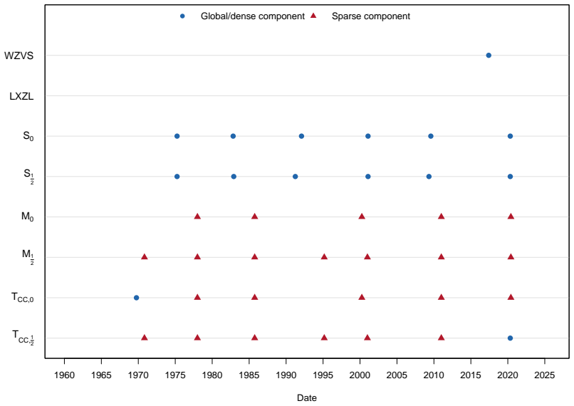
- As a reader inference, the dense and sparse components often select different dates in the empirical panels, suggesting the matched scans can be read as a decomposition of a change into broad shifts and concentrated shifts — a use the paper mentions but does not formalize.
- As a reader inference, a natural extension, pointed to by the paper's own outlook, is a diverging number of changes with shrinking spacing; the fixed-proportion spacing assumption in the WBS theorems is what keeps the shortest-significant selection valid.
Editorial analysis
A structured set of objections, weighed in public.
Referee Report
Summary. The paper proposes sparsity-adaptive tests and localizers for a high-dimensional mean change under temporal dependence. It pairs a quadratic CUSUM scan (dense signal) with a coordinatewise maximum CUSUM scan (sparse signal), under two temporal weightings: an unweighted full scan and a variance-standardized trimmed scan. For each statistic the authors introduce dependence-adjusted centering and long-run scale estimation, prove Gaussian-process or Gumbel null limits, and prove asymptotic independence of the matched quadratic and maximum statistics, which justifies Cauchy combination tests. They also prove single-change localization rates and consistent multiple-change recovery via guarded wild binary segmentation. The paper includes an extensive supplement, simulations for Gaussian and standardized Gamma innovations, and applications to FRED-MD and electricity-load panels.
Significance. If correct, the paper would fill a real gap: joint null calibration of dense and sparse CUSUM scans under non-Gaussian temporal dependence, plus localization and multiple-change recovery within one framework. The supplement is unusually detailed and the simulations are honestly reported, including the explicit concession that the Gamma design lies outside Assumption 1 and the post-hoc white-noise diagnostics showing remaining dependence after mean removal. However, the central "general non-Gaussian" claim rests on Assumption 3, which is not implied by Assumptions 1–2 and fails for a simple temporally independent sub-Gaussian process. In addition, the rate in Theorem 2 contains an impossible term, and the boundary-weighted results are only proved under a growth condition violated by every simulation and application. These issues are load-bearing; the manuscript needs substantial revision before its main claims can be accepted.
major comments (4)
- [Assumption 3 and Lemmas S.3–S.5, S.19, S.24] Assumption 3 is the hinge for the Gaussian comparison steps that produce Theorem 1, Theorem 5, and the WBS theorems, but it is not a consequence of Assumptions 1–2 and it can fail inside the stated framework. Let f_t be iid uniform on [-sqrt(3), sqrt(3)], let eta_{t,j} be iid Rademacher, and set eps_{t,j}=f_t eta_{t,j}. This process is m=0-dependent, projection sub-Gaussian, has Omega=I, and satisfies Assumption 4. For the connected single-block partition in q=2, the blockwise cumulant envelope gives C_{pi,p} = (3/4)p(p-1) - (6/5)p = (3/4)p^2 - (27/20)p = O(p^2), violating Assumption 3. Thus the central theorem's hypotheses are not satisfied by a simple iid sub-Gaussian process, and the claim of covering "general non-Gaussian" dependence is unsupported. The paper gives no primitive sufficient conditions for Assumption 3, and the simulations provide no non-Gaussian evidence: the Gaussian
- [Theorem 2, definition of r_mu,n] The theorem defines r_mu,n = M*sqrt(n) + sqrt(p) M eta_M + ... and asserts r_mu,n -> 0. With M = ceil((n ^ p)^{1/8}), the leading term M*sqrt(n) diverges for every sequence satisfying p = o(n^{3/2}): if p >= n it is at least n^{5/8}, and if p is fixed it is order n^{1/2}. Therefore the stated uniform centering rate cannot be negligible, and the subsequent uses of r_mu,n in Theorem 3 and Theorem 5 are not justified. The proof of Lemma S.10 obtains a stochastic contribution of order M/sqrt(n), so it appears that M/sqrt(n) was intended. If so, correct Theorem 2 and re-verify the feasibility conditions in Theorems 3 and 5; otherwise prove the displayed rate or revise the statement.
- [Theorem 3(ii), Theorem 5, and Section 6/7.1] The boundary-weighted asymptotic statements require log n = o(p^{1/4}). This condition is violated in every simulation and in the FRED-MD application: for n=789, p=119, log n is about 6.67 while p^{1/4} is about 3.30; similarly, n=400, p=250 gives log n ~ 5.99 versus p^{1/4} ~ 3.98, and n=800, p=500 gives 6.68 versus 4.73. Since the boundary-weighted statistics S_{1/2}, M_{1/2}, and T_{CC,1/2} are used and reported as decisive in the applications, the paper is exercising its main calibration tools outside the proven regime. Please either add simulations and applications that satisfy the stated growth condition, or establish the boundary-weighted limits under less restrictive conditions.
- [Simulation Section 6: non-Gaussian coverage of Assumption 3] The only non-Gaussian simulation design is the standardized Gamma innovation, which the paper itself places outside Assumption 1. Thus no simulation demonstrates that Assumption 3 is satisfiable by a non-Gaussian process or that the Gaussian comparison bounds hold beyond the Gaussian-filter case. The empirical size and power results are informative as finite-sample illustrations, but they should not be read as evidence for the general non-Gaussian theorem. Please provide a non-Gaussian simulation within Assumptions 1–3, or state clearly that Assumption 3 is not numerically verified.
minor comments (4)
- [Theorem 2 notation] The term M*sqrt(n) in r_mu,n appears to be a typo for M/sqrt(n). The proof and the claimed convergence suggest the latter; please fix the display and check all places where r_mu,n is used.
- [Sections 2 and 6: Gamma design disclaimer] The statement that the standardized Gamma design is outside Assumption 1 is honest, but the text later says the procedures "retain their sparsity-adaptive behavior under the asymmetric non-Gaussian design." That is a finite-sample claim, not a validation of Theorems 1–5; please make this distinction explicit in the simulation discussion.
- [Section 3 and Section 7: calibration implementation] The RCP preprocessing and finite-LRV tail formulas are described as finite-sample calibration choices not covered by the formal theorems, yet the reported p-values in the applications use them. This is acceptable if clearly labeled, but please add a sentence reminding the reader that the formal theorems apply to the asymptotic p-values, not to the implemented p_FLRV versions.
- [General presentation] The supplement is very long and dense, with many locally defined objects. Adding a short table of notation, especially for the many superscripts on Gaussian analogues (M^{G,gamma}, M^{B,gamma}, M^{eps,gamma}) and for the multiple-change rates, would substantially improve readability.
Circularity Check
No significant circularity: the limiting laws are derived from explicit assumptions; the only self-citation is a published Gaussian-extreme-value theorem used as a tool, not a reduction of the target result to its inputs.
full rationale
The central derivation is conditional on explicit assumptions (Assumptions 1–4) and proves the Gaussian-process, Gumbel, and joint limits via Gaussian comparison, cumulant bounds, and decoupling. The limit covariance of V is obtained from 2 K_B^2 tr(Omega^2)/p after scaling by omega_p, so the law of V is a derived limiting object, not an input or a fitted quantity. The simulated F_V in Remark 1 evaluates that derived covariance, and the Gumbel calibrations are the corresponding limiting distributions. Feasible centering and orientation-complete scaling are proved consistent in Theorem 2; the CF2 correction is proved to be an asymptotically negligible remainder (Lemma S.12), not a fitted correction. The finite-sample LRV tail formulas are explicitly described as computational calibration choices that are not used in the proofs of Theorem 4 or the independence theorems. The closest thing to a self-referential step is the reliance on Wang and Feng (2023) for the Gaussian extreme-value limit and the factorial-moment decoupling argument used in Lemmas S.13 and S.15. Because Wang and Feng is a published theorem on Gaussian processes under Assumption 4-type correlation conditions, and because the present paper records and verifies the relevant decoupling calculation in the supplement, this citation is legitimate independent support rather than a circular reduction to the paper's own conclusion. The more serious concern is that Assumption 3 is a high-level connected-cumulant condition not shown to follow from Assumptions 1–2, and the standardized Gamma design is explicitly outside Assumption 1; that is a coverage and robustness gap, not a circularity in the derivation chain.
Axiom & Free-Parameter Ledger
free parameters (4)
- lambda_n (boundary trimming) =
floor(sqrt(n)) in experiments; theory allows lambda_n ~ n^lambda for any lambda in (0,1)
- M (lag truncation for centering/scale) =
ceil((n∧p)^{1/8})
- LRV bandwidth ell_j =
data-driven; selection rule not specified
- WBS tuning: ell_W,n, N_W,n, d_W,n, Lambda_W =
simulations: 300 intervals, min length 20, guard 95, threshold n^{1/4}; applications unspecified
axioms (7)
- domain assumption Assumption 1: projection sub-Gaussianity plus one of strong mixing (AM), fixed m-dependence (MD), or physical dependence (PD)
- domain assumption Assumption 2: bounded long-run spectrum with p^{-1}tr(Omega^2) -> theta_Omega in (0,infinity) and inf_lambda p^{-1}tr(f_p(lambda)) >= c_f
- domain assumption Assumption 3: connected cumulant contractions max_pi C_{pi,p} <= C_q p for q = 2,3,4
- domain assumption Assumption 4: weak long-run cross-sectional dependence (|rho_jj'| <= rho < 1, sparse near-neighborhood)
- domain assumption Assumption 5: fixed K_cp, Delta_n >= c_Delta n, bounded jumps
- ad hoc to paper Assumption 6: WBS feasibility tuning (ell_W,n, N_W,n, d_W,n, bandwidths)
- standard math Gaussian comparison and extreme-value background (Chernozhukov-Chetverikov-Kato 2013/2017, Leadbetter et al. 1983, Leonov-Shiryaev 1959, Tsirelson 1976, Moricz 1982)
read the original abstract
This paper develops adaptive procedures for detecting and locating mean changes in high-dimensional time series. Quadratic CUSUM statistics target dense changes, whereas coordinatewise maximum statistics target sparse changes. Two weighting schemes are considered to accommodate both interior and boundary changes. Under general non-Gaussian vector dependence, we establish the limiting distributions, validate the required centering and scaling estimators, and prove asymptotic independence between matched quadratic and maximum statistics. These results justify Cauchy combination tests. We further establish single-change localization and consistent multiple-change recovery using wild binary segmentation. Numerical results illustrate the effectiveness of the proposed methods.
Figures



Reference graph
Works this paper leans on
-
[1]
Adler, R. J. and J. E. Taylor (2007).Random Fields and Geometry. Springer
2007
-
[2]
Aston, J. A. D. and C. Kirch (2018). High dimensional efficiency with applications to change point tests.Electronic Journal of Statistics 12(1), 1901–1947
2018
-
[3]
Bai, J. (2010). Common breaks in means and variances for panel data.Journal of Econometrics 157(1), 78–92
2010
-
[4]
Chen, and P
Baranowski, R., Y. Chen, and P. Fryzlewicz (2019). Narrowest-over-threshold detection of multiple change points and change-point-like features.Journal of the Royal Statistical Society: Series B (Statistical Methodology) 81(3), 649–672
2019
-
[5]
(2013).Convergence of Probability Measures
Billingsley, P. (2013).Convergence of Probability Measures. Wiley
2013
-
[6]
Chan, K. W. (2022). Optimal difference-based variance estimators in time series: A general framework.The Annals of Statistics 50(3), 1376–1400
2022
-
[7]
Chen, and M
Chang, J., X. Chen, and M. Wu (2024). Central limit theorems for high dimensional dependent data.Bernoulli 30(1), 712–742
2024
-
[8]
Chang, J., J. He, C. Lin, and Q. Yao (2024). HDTSA: An R package for high-dimensional time series analysis. arXiv preprint arXiv:2412.17341
Pith/arXiv arXiv 2024
-
[9]
Wang, and W
Chen, L., W. Wang, and W. B. Wu (2022). Inference of breakpoints in high-dimensional time series.Journal of the American Statistical Association 117(540), 1951–1963
2022
-
[10]
Chetverikov, and K
Chernozhukov, V., D. Chetverikov, and K. Kato (2013). Gaussian approximations and multiplier bootstrap for maxima of sums of high-dimensional random vectors.The Annals of Statistics 41(6), 2786–2819
2013
-
[11]
Chetverikov, and K
Chernozhukov, V., D. Chetverikov, and K. Kato (2017). Central limit theorems and bootstrap in high dimensions. The Annals of Probability 45(4), 2309–2352
2017
-
[12]
Cho, H. (2016). Change-point detection in panel data via double CUSUM statistic.Electronic Journal of Statistics 10(2), 2000–2038
2016
-
[13]
Davydov, Y. A. (1968). Convergence of distributions generated by stationary stochastic processes.Theory of Probability and Its Applications 13(4), 691–696
1968
-
[14]
Enikeeva, F. and Z. Harchaoui (2019). High-dimensional change-point detection under sparse alternatives.The Annals of Statistics 47(4), 2051–2079
2019
-
[15]
Fryzlewicz, P. (2014). Wild binary segmentation for multiple change-point detection.The Annals of Statistics 42(6), 2243–2281. Horv´ath, L. and M. Huˇskov´a (2012). Change-point detection in panel data.Journal of Time Series Analysis 33(4), 631–648
2014
-
[16]
(1997).Gaussian Hilbert Spaces
Janson, S. (1997).Gaussian Hilbert Spaces. Cambridge: Cambridge University Press
1997
-
[17]
Jin, B., G. Pan, Q. Yang, and W. Zhou (2016). On high-dimensional change point problem.Science China Mathematics 59(12), 2355–2378
2016
-
[18]
Jirak, M. (2015). Uniform change point tests in high dimension.The Annals of Statistics 43(6), 2451–2483
2015
-
[19]
Leadbetter, M. R., G. Lindgren, and H. Rootz ´en (1983).Extremes and Related Properties of Random Sequences and Processes. New York: Springer
1983
-
[20]
Leonov, V. P. and A. N. Shiryaev (1959). On a method of calculation of semi-invariants.Theory of Probability and Its Applications 4(3), 319–329
1959
-
[21]
Li, J., M. Xu, P.-S. Zhong, and L. Li (2019). Change point detection in the mean of high-dimensional time series data under dependence.arXiv preprint arXiv:1903.07006. 105
Pith/arXiv arXiv 2019
-
[22]
Zhang, and Y
Liu, B., X. Zhang, and Y. Liu (2022). High dimensional change point inference: Recent developments and extensions.Journal of Multivariate Analysis 188, 104833
2022
-
[23]
Liu, B., C. Zhou, X. Zhang, and Y. Liu (2020). A unified data-adaptive framework for high dimensional change point detection.Journal of the Royal Statistical Society: Series B 82(4), 933–963
2020
-
[24]
Gao, and R
Liu, H., C. Gao, and R. J. Samworth (2021). Minimax rates in sparse, high-dimensional change point detection. The Annals of Statistics 49(2), 1081–1112
2021
-
[25]
McCracken, M. W. and S. Ng (2016). FRED-MD: A monthly database for macroeconomic research.Journal of Business & Economic Statistics 34(4), 574–589
2016
-
[26]
Peligrad, and E
Merlev`ede, F., M. Peligrad, and E. Rio (2011). A bernstein type inequality and moderate deviations for weakly dependent sequences.Probability Theory and Related Fields 151(3–4), 435–474. M´oricz, F. (1982). A general moment inequality for the maximum of partial sums of single series.Acta Scientiarum Mathematicarum 44(1–2), 67–75
2011
-
[27]
Carpentier, and N
Pilliat, E., A. Carpentier, and N. Verzelen (2023). Optimal multiple change-point detection for high-dimensional data.Electronic Journal of Statistics 17(1), 1240–1315
2023
-
[28]
Saulis, L. and V. A. Statuleviˇcius (1991).Limit Theorems for Large Deviations. Dordrecht: Springer
1991
-
[29]
Trindade, A. (2015). ElectricityLoadDiagrams20112014. UCI Machine Learning Repository. Dataset
2015
-
[30]
Tsirelson, V. S. (1976). The density of the distribution of the maximum of a gaussian process.Theory of Probability and Its Applications 20(4), 847–856
1976
-
[31]
Wang, G. and L. Feng (2023). Computationally efficient and data-adaptive changepoint inference in high dimension. Journal of the Royal Statistical Society: Series B 85(3), 936–958
2023
-
[32]
Zou, and G
Wang, G., C. Zou, and G. Yin (2018). Change-point detection in multinomial data with a large number of categories.The Annals of Statistics 46(5), 2020–2044
2018
-
[33]
Wang, R. and X. Shao (2023). Dating the break in high-dimensional data.Bernoulli 29(4), 2879–2901
2023
-
[34]
Wang, R., C. Zhu, S. Volgushev, and X. Shao (2022). Inference for change points in high-dimensional data via self-normalization.The Annals of Statistics 50(2), 781–806
2022
-
[35]
Wang, T. and R. J. Samworth (2018). High dimensional change point estimation via sparse projection.Journal of the Royal Statistical Society: Series B 80(1), 57–83
2018
-
[36]
Wang, Y., C. Zou, Z. Wang, and G. Yin (2019). Multiple change-points detection in high dimension.Random Matrices: Theory and Applications 8(4), 1950014
2019
-
[37]
Wu, W. B. (2005). Nonlinear system theory: Another look at dependence.Proceedings of the National Academy of Sciences of the United States of America 102(40), 14150–14154
2005
-
[38]
Wu, W. B. and Y. N. Wu (2016). Performance bounds for parameter estimates of high-dimensional linear models with correlated errors.Electronic Journal of Statistics 10(1), 352–379
2016
-
[39]
Yu, M. and X. Chen (2021). Finite sample change point inference and identification for high-dimensional mean vectors.Journal of the Royal Statistical Society: Series B 83(2), 247–270
2021
-
[40]
Wang, and X
Zhang, Y., R. Wang, and X. Shao (2022). Adaptive inference for change points in high-dimensional data.Journal of the American Statistical Association 117(540), 1751–1762. 106
2022
discussion (0)
Sign in with ORCID, Apple, or X to comment. Anyone can read and Pith papers without signing in.