REVIEW 3 major objections 5 minor 24 references
On a cross coupling of Rulkov neural maps
T0 review · 3 major / 5 minor · reviewed 2026-08-01 · deepseek-v4-flash
Pith's one-line read A new cross coupling of two Rulkov neuron maps exchanges their fast-variable inputs, and the paper proves the 4D system preserves bounded motion and inherits a snap-back repeller — hence Devaney chaos — when the 2D map has one.
desk verdict New cross-coupling of Rulkov maps with a clean boundedness proof and rich numerics, but the snap-back repeller inheritance theorem rests on an invalid decoupling assumption in the proof. read the letter →
The pith
A machine-rendered reading of the paper's core claim, the machinery that carries it, and where it could break.
The reading
What carries the argument
The load-bearing object is the cross-coupling map C:R^4→R^4 given by (2), which can be written as x_{n+1}=A x_n+b(x_n) with A block-diagonal and b bounded. The eigenvalues of A are (1±√(1−4μ))/2 and (1±√(1−4ν))/2, so for μ,ν<1/2 a theorem on linear-plus-bounded perturbations yields an absorbing set. For the chaotic persistence result, the key structure is the product form of the snap-back repeller: the 2D repelling neighborhood B_r(p0) is lifted to B_r(p0)×B_{r+ε}(p0) in R^4, and the returning point q̃0=(x,y,x+ε1,y+ε2) is tuned so that after k iterations it hits the lifted fixed point; the solvability of the resulting equations (37)–(39) is attributed to the implicit function theorem. A snap
What would settle it
For a parameter set satisfying Theorem 4's hypotheses, compute the Jacobian of the coupled map at the proposed fixed point p̃0; if any eigenvalue has modulus below 1, p̃0 is not repelling and cannot anchor a snap-back repeller. Alternatively, solve equations (37)–(39) numerically for ε1, ε2 and check that the resulting q̃0 lies in B~, that C^(k)(q̃0)=p̃0, and that det(DC^j(q̃0))≠0 for j=1,...,k; failure of any of these checks would refute the construction.
Extended reading notes
Core claim
The paper's central claim is that the cross-coupling map (2), defined by x_{n+1}=αf(z_n)+y_n, y_{n+1}=y_n−μ(x_n−σ), z_{n+1}=βf(x_n)+ω_n, ω_{n+1}=ω_n−ν(z_n−ρ), inherits the two main dynamical guarantees of the uncoupled Rulkov map. Theorem 3 proves that if the 2D map has an absorbing set and μ=ν, then the 4D map has an absorbing set, so all orbits are eventually bounded. Theorem 4 proves that if the 2D map has a snap-back repeller, σ=ρ, and the coupled map has a repelling fixed point, then the 4D map also has a snap-back repeller, which by the Marotto theorem implies chaos in the sense of Devaney. For the standard chaotic Rulkov choice f(x)=1/(1+x^2), the paper notes that Theorem 4 does not a
Load-bearing premise
The load-bearing premise is that equations (37)–(39) can be solved for ε1, ε2 inside the repelling neighborhood B~ by the implicit function theorem; the paper does not verify that the relevant Jacobian is nonsingular or that the solution remains in B~, and without that the 4D map need not have a snap-back repeller (and for f(x)=1/(1+x^2) the theorem does not apply at all because the coupled map has no repelling fixed point).
Editorial extensions
If this is right
- If the original 2D Rulkov map has an absorbing set and μ=ν, every orbit of the 4D cross-coupled system eventually enters a fixed compact region, so the coupling cannot produce unbounded motion.
- If the original map has a snap-back repeller, the coupled map has a repelling fixed point, and σ=ρ, then the 4D map inherits a snap-back repeller and is chaotic in the Devaney sense by the Marotto theorem.
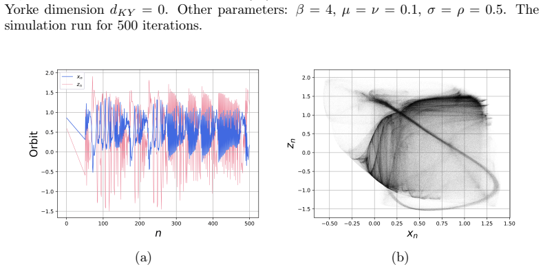
- For the standard chaotic Rulkov nonlinearity f(x)=1/(1+x^2), the numerical results (dKY near 1.8, positive maximum Lyapunov exponent, fractal basins) indicate that the chaotic regime persists under cross coupling even though the analytical snap-back-repeller theorem does not apply.
- In the small-perturbation regime μ,ν≪1, the coupled model reproduces the bursting-firing time series of a single Rulkov neuron, so the coupling is a plausible two-neuron map.
- Because the absorbing-set proof only uses boundedness of f, the same construction should transfer to any continuous bounded map-based neuron model, not only Rulkov's.
Reading between the lines
- Editorial inference: the same absorbing-set argument should carry over to any cross coupling of two fast-slow maps with bounded response and linear slow dynamics, so the template is broader than Rulkov's model; this is a transfer, not a result the paper proves.
- Editorial inference: the numerical strange attractor for the standard Rulkov nonlinearity, where the theorem is explicitly inapplicable, suggests the repelling-fixed-point obstruction may be an artifact of the proof technique; looking for another chaos certificate (e.g., a direct 4D snap-back repeller or positive Lyapunov dimension) would resolve whether the analytical gap is real or just technica
- Editorial inference: the claimed biological reading of the μ,ν≲1 regime as two brain-region frontiers is heuristic; a testable consequence is that statistical features of the time series (spike counts, inter-spike intervals, synchronization measures) should separate clearly between the small- and large-perturbation regimes.
- Editorial inference: the proposed N-neuron generalization (41) is where the approach would prove its worth; if the absorbing-set proof extends to N, it gives a straightforward way to grow provably bounded, chaotic neural networks, but the paper does not yet provide that extension.
Signed reviews
Editorial analysis
A structured set of objections, weighed in public.
Referee Report
Summary. The paper introduces a four-dimensional 'cross coupling' of two Rulkov neural maps, in which the fast variable of each neuron is driven by the other neuron's fast variable. The authors claim to prove analytically that this coupling preserves boundedness of motion (via an absorbing set) and, under additional hypotheses, inherits a snap-back repeller from the two-dimensional Rulkov map, thereby implying Devaney chaos through the Marotto theorem. Numerical experiments for the standard nonlinearity f(x)=1/(1+x^2) report a strange attractor with Kaplan-Yorke dimension ≈1.8, Lyapunov spectra, bifurcation diagrams, and fractal basins of attraction. The paper also sketches a generalization to N coupled neurons.
Significance. If the analytic results were correct, they would provide a rigorous route to Devaney chaos in a four-dimensional coupled neuron model and a clean boundedness criterion. The boundedness result for μ,ν∈(0,1/2) (Corollary 1) is a correct and appealing application of Ortega's bounded-perturbation lemma, and the numerical study is extensive and reproducible in structure. However, the main analytic theorem on snap-back repeller inheritance is not established as proven, and the paper itself notes that the theorem does not apply to the standard Rulkov nonlinearity used in the numerics. This substantially weakens the claimed analytical contribution, leaving the boundedness result for a restricted parameter range and numerical evidence as the principal content.
major comments (3)
- [Theorem 4, Eq. (36)–(39)] The proof assumes that the first two components of the k-th iterate of the coupled map depend only on the first two arguments, and the last two only on the last two. For the cross-coupled system this is false for k≥2. For example, with k=2, x_2 = α f(β f(x_0)+ω_0) + y_0 − μ(x_0−σ), which depends on ω_0; for k≥3 the dependence includes all four initial variables. Hence the identity C_1^(k)(x,y,x+ε_1,ε_2)=C_1^(k)(x,y) does not hold, and the first two components of C^k( q̃_0) are not automatically (p_0x,p_0y). The implicit-function-theorem step (37)–(39) solves only two equations while four must be satisfied; no Jacobian nonsingularity condition is verified and no argument ensures the solution remains in B̃. The same reasoning is then extended to μ≠ν without proof. This invalidates the claimed construction of a snap-back repeller for the coupled map and the resulting Devaney-chaos conclusio
- [Theorem 3, Eqs. (18)–(29)] The comparison argument for the y and ω components is not valid. Since y_{n+1}=y_n − μ(x_n−σ), if the upper-control system has X_n ≥ x_n, then Y_{n+1}=Y_n − μ(X_n−σ) ≤ y_{n+1} for equal initial data. Thus the upper control's y-component is a lower bound, not an upper bound, for the original y. Consequently the statement that the motion is 'confined ... below and on the left' of the rectangle (22) is incorrect, and the claimed upper bound y ≤ b+M_1 is not obtained. The lower bound y ≥ a−M_3 is similarly unsupported. Therefore the boundedness claim for μ,ν∈(1/2,1) is not established; Corollary 1, which covers μ,ν∈(0,1/2), is not affected.
- [Corollary 2] The corollary invokes persistence of snap-back repellers under small C^1 perturbations [15]. The coupled map is not shown to be a small C^1 perturbation of the uncoupled system: the smallness of σ−ρ does not control α−β or μ−ν, and the coupling terms are O(1) in f. Moreover, Theorem 4 already requires the coupled system to have a repelling fixed point, and the perturbation statement does not verify that condition. The corollary is therefore not supported by the cited persistence theorem.
minor comments (5)
- [Eq. (38)] The equation 'R_2^(k)(x+ε_1,y+ε_2)=p_0y+ε' appears to misidentify the ω-component of the coupled map with the y-component of the two-dimensional map; this is at least a typo and should be corrected.
- [Lemma 1] The proof uses a norm notation that is ambiguous; a componentwise bound is simpler and sufficient. The statement itself is correct.
- [Data availability] The statement 'The data that supports the funding of this study are available within the article' seems to contain a typo ('funding' should likely be 'findings'). No code or data repository is provided.
- [Theorem 2] Theorem 2 is attributed to Ortega, 2026, but no corresponding reference entry appears in the bibliography; please add a full citation or a note on the communication.
- [Notation] The space C^0_b(R) is used without definition; it should be defined as the space of continuous bounded functions.
Circularity Check
No significant circularity: the analytical transfer theorems use external mathematical results and explicit constructions, and the numerical evidence is not fitted to force the conclusion.
full rationale
The paper's central analytical claims are transfer statements: Theorem 3 proves that an absorbing set for the 2D Rulkov map implies an absorbing set for the 4D cross-coupled system, using a communicated linear-perturbation lemma (Ortega 2026) and a translation argument; Theorem 4 aims to inherit a snap-back repeller from the 2D system to the 4D system, invoking Marotto's theorem and an external 2D snap-back repeller result [14], plus a persistence result [15]. No parameter is fitted and then renamed as a prediction; the Kaplan-Yorke dimension is computed from Lyapunov exponents rather than imposed. The proof of Theorem 4 does contain a serious rigor gap: the claimed implicit-function-theorem solvability of equations (37)-(39) is not verified, and the decoupling structure assumed in (36) is not valid for iterates k≥2. However, that is a correctness/rigor concern, not circularity: the theorem's conclusion is not equivalent to its hypotheses by definition, and no step reduces to a self-citation or to a fitted input. The paper even flags that Theorem 4 does not apply to the standard chaotic Rulkov case, which further weakens the analytical bridge without making it circular. Thus the circularity score is 0.
Assumptions & free parameters
free parameters (1)
- Numerical parameter set for the reported strange attractor =
alpha=1.1, beta=4, mu=nu=0.1, sigma=rho=0.5
assumptions (7)
- domain assumption f in C^0_b(R), in particular f(x)=1/(1+x^2) is bounded and continuous
- standard math Marotto theorem: a snap-back repeller implies Devaney chaos
- domain assumption Kaplan-Yorke dimension estimates the fractal dimension of the attractor
- standard math Persistence of a snap-back repeller under small C^1 perturbations (ref [15])
- ad hoc to paper Implicit function theorem solvability of equations (37)-(39) inside the repelling neighborhood
- domain assumption The original Rulkov map (1) has a snap-back repeller in the chaotic parameter regime (ref [14])
- domain assumption The cross-coupling (2) has a repelling fixed point
Cite this review
Pith. "Pith review of On a cross coupling of Rulkov neural maps." pith.science (2026). https://pith.science/paper/IVBQRSOX
@misc{pith2026260722318,
  author       = {Pith},
  title        = {Pith review of: On a cross coupling of Rulkov neural maps},
  year         = {2026},
  howpublished = {\url{https://pith.science/paper/IVBQRSOX}},
  note         = {Machine review of arXiv:2607.22318}
}
read the original abstract
We introduce a novel coupling of Rulkov neural maps, proposing a heuristic biological interpretation for the transition to non-small values of the perturbations acting on the slow variables. We analytically prove that the coupling preserves boundedness of motion and the existence of a snap-back repeller (leading to Devaney chaos by the Marotto theorem), if they are associated to the original system. For the coupling of two standard chaotic Rulkov maps, we present numerical simulations for the orbits of the system showing the arising of a global strange attractor, whose fractal structure is strongly suggested by the computation of a non-integer Kaplan-Yorke dimension. Furthermore, we perform standard numerical studies concerning time series, Lyapunov exponents spectra, bifurcation diagrams and basins of attraction. Finally, we briefly propose a generalization of the coupling to an arbitrary number of neurons.
Figures


Figures from the paper (11 more)



Reference graph
Works this paper leans on
-
[15]
Y. Chen, Y. Huang, L. Li, The persistence of snap-back repeller under smallC 1 perturbations in Banach spaces, International Jour- nal of Bifurcation and Chaos 21 (3) (2011) 703–710.doi:10.1142/ S0218127411028702
2011
-
[1]
A. L. Hodgkin, A. F. Huxley, A quantitative description of membrane current and its application to conduction and excitation in nerve, J. Physiol. 117 (1952) 500–544.doi:10.1113/jphysiol.1952.sp004764
-
[2]
Chialvo, Generic excitable dynamics on a two-dimensional map, Chaos, Solitons&Fractals 5 (1995) 461–479.doi:10.1016/ 0960-0779(93)E0056-H
D. Chialvo, Generic excitable dynamics on a two-dimensional map, Chaos, Solitons&Fractals 5 (1995) 461–479.doi:10.1016/ 0960-0779(93)E0056-H
1995
-
[3]
E. M. Izhikevich, Simple model of spiking neurons, IEEE Trans. Neural Netw. 14 (2003) 1569–1572.doi:10.1109/TNN.2003.820440
arXiv 2003
-
[4]
N. F. Rulkov, Modeling of spiking-bursting neural behavior using two- dimensional map, Phys. Rev. E 65 (2002) 041922.doi:10.1103/ PhysRevE.65.041922
2002
-
[5]
B.Ibarz, J.M.Casado, M.A.F.Sanjuán, Map-basedmodelsinneuronal dynamics, Physics Reports 501 (2011) 1–74.doi:10.1016/j.physrep. 2010.12.003. 24
-
[6]
S. Rakshit, A. Ray, B. K. Bera, D. Ghosh, Synchronization and firing patterns of coupled Rulkov neuronal map, Nonlinear Dyn. 94 (2018) 785–805.doi:10.1007/s11071-018-4394-8
-
[7]
S. Mirzaei, M. Mehrabbeik, K. Rajagopal, S. Jafari, G. Chen, Synchro- nization of a higher-order network of Rulkov maps, Chaos 32 (2022) 123133.doi:10.1063/5.0117473
Show all 24 references
-
[8]
F. R. Marotto, Snap-Back Repellers Imply Chaos inR n, Journal of Mathematical Analysis and Applications 63 (1978) 199–223.doi: 10.1016/0022-247X(78)90115-4
1978 doi
-
[9]
F. R. Marotto, On redefining a snap-back repeller, Chaos, Solitons& Fractals 25 (2005) 25–28.doi:10.1016/j.chaos.2004.10.003
2005 doi
-
[10]
R. L. Devaney, An Introduction to Chaotic Dynamical Systems, 2nd ed., Addison-Wesley, Redwood City, CA, 1989
1989
-
[11]
T.-Y. Li, J. A. Yorke, Period three implies chaos, Am. Math. Mon. 82 (10) (1975) 985–992.doi:10.2307/2318254
1975 doi
-
[12]
Y. Shi, G. Chen, Discrete chaos in Banach spaces, Sci. China Ser. A Math. 48 (2) (2005) 222–238.doi:10.1360/03ys0183
2005 doi
-
[13]
Banks, J
J. Banks, J. Brooks, G. Cairns, G. Davis, P. Stacey, On Devaney’s definition of chaos, The American Mathematical Monthly 99 (4) (1992) 332–334.doi:10.2307/2324899
1992 doi
-
[14]
P. Ge, H. Cao, Chaos in the Rulkov Neuron Model Based on Marotto’s Theorem, International Journal of Bifurcation and Chaos 31 (15) (2021) 2150233.doi:10.1142/S0218127421502333
2021 doi
-
[16]
M. R. Guevara, L. Glass, Phase Locking, Period Doubling Bifurcations and Chaos in a Mathematical Model of a Periodically Driven Oscilla- tor: A Theory for the Entrainment of Biological Oscillators and the Generation of Cardiac Dysrhythmias., J. Math. Biology 14 (1982) 1–23. do...
1982 doi
-
[17]
Kaplan, J
J. Kaplan, J. Yorke, Chaotic behavior of multidimensional difference equations, In: Peitgen, H. O.; Walther, H. O. (eds.), Functional Differ- ential Equations and the Approximation of Fixed Points. Lecture Notes in Mathematics 730 (1979) 204–227.doi:10.1007/BFb0064319
1979 doi
-
[18]
B. B. Le, N. A. Gandhi, Exploring Geometrical Properties of Chaotic Systems Through an Analysis of the Rulkov Neuron MapsarXiv:2406.08385v2 (2024)
2024 arXiv
-
[19]
A. N. Pisarchik, U. Feudel, Control of multistability, Physics Reports 540 (4) (2014) 167–218.doi:10.1016/j.physrep.2014.02.007
2014 doi
-
[20]
Wagemakers, Basins of Attraction: A Dynamical Zoo, International Journal of Bifurcation and Chaos 35 (11) (2025) 2530024.doi:10.1142/ S0218127425300241
A. Wagemakers, Basins of Attraction: A Dynamical Zoo, International Journal of Bifurcation and Chaos 35 (11) (2025) 2530024.doi:10.1142/ S0218127425300241
2025
-
[21]
Boccaletti, J
S. Boccaletti, J. Kurths, G. Osipov, V. D. L., C. S. Zhou, The syn- chronization of chaotic systems, Physics Report 366 (2002) 1–101. doi:10.1016/S0370-1573(02)00137-0
2002 doi
-
[22]
Arnold, Random Dynamical Systems, Springer Monographs in Math- ematics, Springer-Verlag, Berlin Heidelberg, 1998.doi:10.1007/ 978-3-662-12878-7
L. Arnold, Random Dynamical Systems, Springer Monographs in Math- ematics, Springer-Verlag, Berlin Heidelberg, 1998.doi:10.1007/ 978-3-662-12878-7
1998
-
[23]
Pilarczyk, G
P. Pilarczyk, G. Graff, An absorbing set for the Chialvo map, Commun. Nonlinear Sci. Numer. Simulat. 132 (2024) 107947.doi:10.1016/j. cnsns.2024.107947
2024
-
[24]
Tanaka, M
G. Tanaka, M. A. F. Sanjuán, K. Aihara, Crisis-induced intermittency in two coupled chaotic maps: Towards understanding chaotic itiner- ancy, Physical Review E 71 (2005) 016219.doi:10.1103/PhysRevE. 71.016219. 26
2005 doi
Reviewed August 1, 2026 · model on record in the stance chip above.
Discussion (0). Continue with ORCID to comment.