REVIEW 3 major objections 8 minor 72 references
Atmospheric Escape Rates of Planets in Stellar Tidal Fields from 3-D Hydrodynamic Simulations
T0 review · 3 major / 8 minor · reviewed 2026-07-31 · grok-4.5
Pith's one-line read A mixture of spherical and tidal-tail escape formulas, trained on 3D runs, beats 1D Parker models for planetary mass-loss rates.
desk verdict Solid 3D regime map of tidal vs thermal escape; the Mixture Model is a useful in-grid fit but its flashiest population corrections rest on unvalidated extrapolation of g(λ_p). read the letter →
The pith
A machine-rendered reading of the paper's core claim, the machinery that carries it, and where it could break.
The reading
What carries the argument
The Mixture Model: a weighted geometric mean of a modified spherical Parker wind and a modified tidal two-tail (nozzle) rate, with the weight set by a sigmoid of the hydrodynamic escape parameter and the dimensionless L1 barrier height, calibrated directly on the 3D simulation grid.
What would settle it
Run the same 3D setup at a handful of points inside the grid with a realistic energy equation (photoionization heating, radiative cooling, multi-species chemistry) and check whether the Mixture Model still recovers the measured mass-loss rates to the same accuracy.
Extended reading notes
Core claim
Three-dimensional hydrodynamic simulations of thermally driven planetary outflows demonstrate that mass-loss morphology and rate transition smoothly from nearly isotropic Parker-like winds (weak tides, hot atmospheres) to anisotropic two-tailed streams through the Lagrange points (strong tides, cooler atmospheres). A calibrated Mixture Model that geometrically averages a modified spherical Parker rate and a modified L1/L2 nozzle rate reproduces the simulated mass-loss rates across the explored grid and outperforms both pure Parker and tidally corrected 1D models.
Load-bearing premise
The entire thermodynamic state of the atmosphere is collapsed to a single nearly isothermal sound speed with fixed surface density and no stellar wind, magnetic fields, or detailed heating and cooling.
Editorial extensions
If this is right
- Most observed close-in planets lie where Parker and Mixture rates differ by less than 30 percent, so existing demographic calculations remain first-order safe.
- A minority of strongly Roche-filling, tightly bound systems can have true mass-loss rates several times higher than pure Parker estimates.
- A larger minority of hot, loosely bound small planets can have true rates far lower than pure Parker estimates, affecting radius-valley and desert models.
- Mean radial density profiles from 1D tidal codes remain usable even when the flow is anisotropic; only the angular structure is lost.
Reading between the lines
- Coupling the Mixture Model into long-term orbital and structural evolution codes would change predicted lifetimes most for the hottest, lowest-mass close-in planets and for near-Roche-lobe gas giants.
- Transit spectroscopy of leading versus trailing tails could observationally flag the strong-tide regime where the Mixture weight approaches unity.
- Extending the calibration grid below λ_p ≈ 2.5 and above ≈ 7.5 would immediately widen the model’s safe domain for super-Earths and cooler giants.
Editorial analysis
A structured set of objections, weighed in public.
Referee Report
Summary. The paper presents a suite of 45 three-dimensional hydrodynamic simulations (Athena++), on a grid of Roche-lobe-filling factor f_ϕ ∈ [0.01, 5] and hydrodynamic escape parameter λ_p ∈ {2.5, 5, 7.5}, of thermal atmospheric outflows from a Jupiter-mass planet in the corotating Roche potential of a solar-mass star. The authors document a smooth morphological transition from quasi-spherical, isotropic winds (weak tides, hot outflows) to anisotropic two-tail escape through the L1/L2 channels (strong tides, cool outflows), supported by density maps, Mach-number/sonic-surface maps, and angular mass-flux distributions on the Hill sphere (Figs. 1–3). They then compare measured mass-loss rates with five analytic models — Parker wind, an empirically corrected "Modified Spherical" model, an L1/L2 "Nozzle" model, a "Modified Tidal Two-Tail" model with a fitted L2 attenuation, and the p-winds 1D tidal model — and combine the spherical and tidal limits into a "Mixture Model" (a logistic-weighted geometric mean) calibrated on the same simulation grid. Finally, they apply the Mixture Model to the observed exoplanet population using sunset-catalog outflow temperatures, finding that the Parker wind agrees with the Mixture Model for ~84% of planets but can deviate strongly for tide-dominated tightly bound systems and for hot, loosely bound ones.
Significance. If the simulation results hold, this is a useful and timely contribution. Hydrodynamic escape rates remain uncertain at the order-of-magnitude level in population studies, and a systematic 3D benchmark isolating tidal effects is directly relevant to interpreting the radius valley, the hot-Neptune desert, and He 1083 nm / Lyα transit observations. Notable strengths: a 45-run grid with a resolution convergence test (Appendix A) and a surface-integral Ṁ diagnostic verified to be radius-independent over 0.2–0.5a; explicit, equation-level comparisons against Parker, modified-spherical, nozzle, modified-tail, and 1D tidal (p-winds) models; and an open-source implementation of the Mixture Model with the full mass-loss table archived on Zenodo, making the results reproducible and the model falsifiable against future simulations. The morphology diagnostics (spherical-to-two-tail transition, sonic-surface deformation, angular flux maps) are robust, non-circular outputs of the hydro runs and constitute, in my view, the paper's most durable contribution. The credibility of the population-level application in §5.1, however, depends on resolving the extrapolation and in-sample-validation issues
major comments (3)
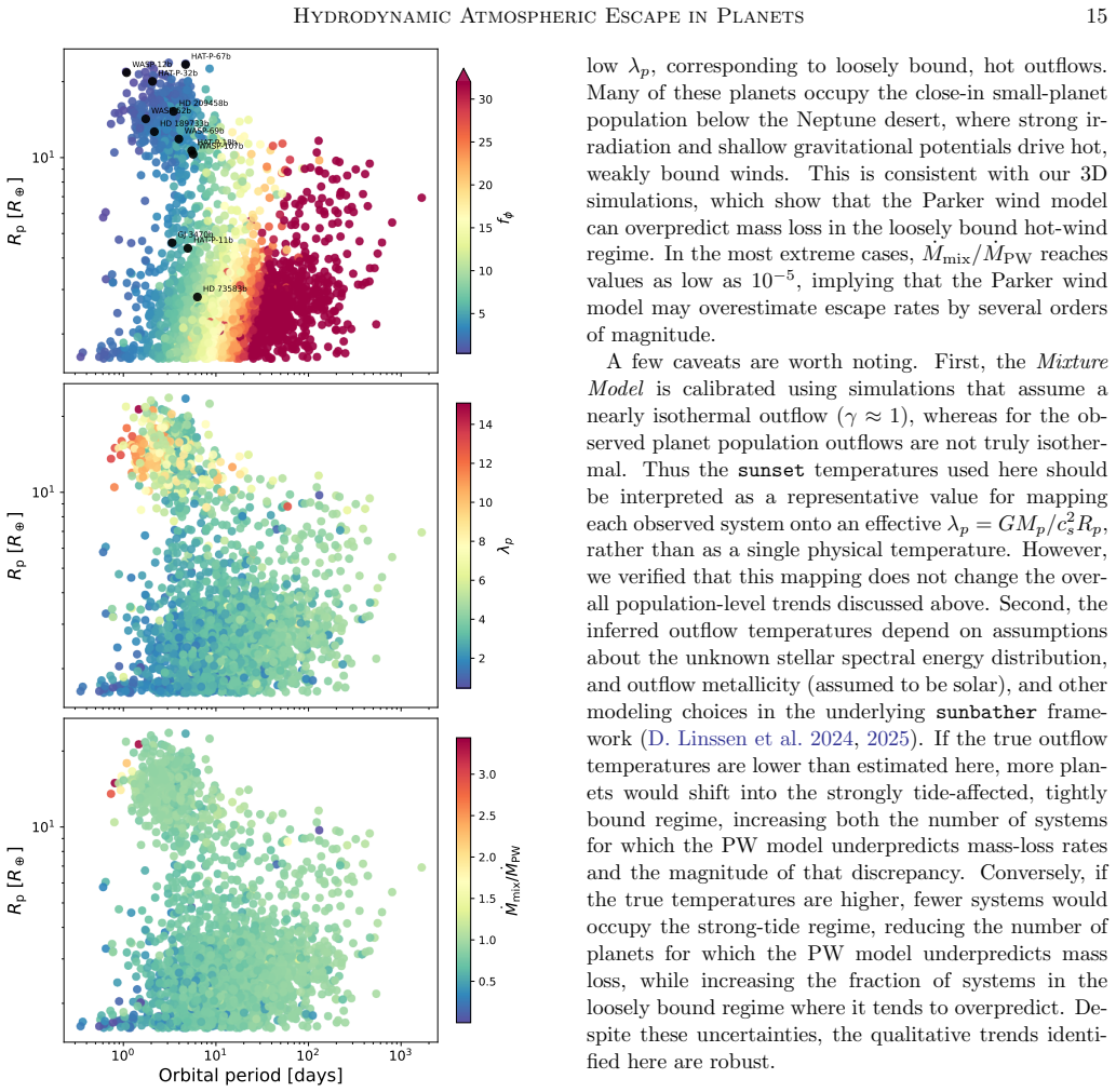
- [§5.1, Fig. 6 (bottom); Eq. (13)] The most dramatic application result — the bottom panel of Fig. 6 and the statement in §5.1 that 'Ṁ_mix/Ṁ_PW reaches values as low as 10^-5, implying that the Parker wind model may overestimate escape rates by several orders of magnitude' — is generated entirely by extrapolating the empirical correction g(λ_p)=exp(−k_sph/λ_p²) with k_sph=2.47 below the calibrated range. The simulated grid spans only 2.5≤λ_p≤7.5 (Table 1), over which g varies modestly (0.67–0.96). For the small-λ_p, low-η planets in question, the fitted logit (β0=−7.00, β1=6.13, β2=−4.03) drives w→0, so Ṁ_mix→g(λ_p)Ṁ_PW; at λ_p≈0.5 this gives exp(−2.47/0.25)≈5×10^-5 — i.e., the headline correction is numerically identical to the value of an unvalidated exponential at λ_p values never simulated. Worse, for λ_p<2 the isothermal Parker sonic radius r_s=R_p(λ_p/2) (§3.2) lies inside the planet, so no transonic Parker solution
- [§4.1–4.4, Fig. 4, Table 2] The central claim that the Mixture Model 'accurately predicts mass-loss rates across the parameter space explored and outperforms 1D model with tidal corrections' (Abstract; §4.4; Fig. 4) is established entirely in-sample. Five free parameters (k_sph, k_tail, β0, β1, β2) are least-squares fit to the same 45 Ṁ_sim values listed in Table 1 and then plotted against those same values in Fig. 4. With only three λ_p rows and smooth monotonic trends in f_ϕ, a five-parameter smooth interpolant is nearly guaranteed to agree, so Fig. 4 is a demonstration of fitting, not of predictive performance. A minimal fix that would substantially strengthen the paper: a hold-out test, e.g., calibrate on two of the three λ_p rows (or a subset of f_ϕ values) and predict the withheld runs. At minimum the authors should report per-point residuals, soften 'accurately predicts'/'outperforms' to reflect in-sample ca
- [§4.1, Eq. (13); §4.2, Eq. (17)] The functional form g(λ_p)=exp(−k_sph/λ_p²) is introduced without justification beyond the qualitative statement that the sonic point lies close to the surface at small λ_p. Within the grid, k_sph=2.47 is constrained almost entirely by the λ_p=2.5 row: at λ_p=5 and 7.5 the unmodified PW already under- or matches-predicts (Table 1), so the λ_p-dependence of g is essentially unconstrained by the data — yet it is this unconstrained λ_p-dependence that dominates the low-λ_p extrapolation behind Major Comment 1. The same concern applies, more mildly, to h(λ_p)=exp(−k_tail/Ro²): the claimed Ro^-2 scaling of the L2 suppression is motivated by a physical argument (§4.2) but the functional form is one of many consistent with the grid. Please report the fit residuals as a function of λ_p for both corrections, and either demonstrate that alternative forms (e.g., g constant, g∝exp(−k/λ_p)) are disfa
minor comments (8)
- [Table 1] First data row: for (f_ϕ=0.010, λ_p=2.50), Ṁ_sim is listed as 1.00×10^-4 while the adjacent rows are ~9.9×10^-4 and Ṁ_mix=9.86×10^-4 exceeds it by an order of magnitude. This appears to be a typo for 1.00×10^-3; since Table 1 is the benchmark dataset (and is distributed on Zenodo), please verify.
- [§5.2 / Fig. 7 caption] The text twice refers to 'Figure 3 (blue curve)' and 'Figure 3, left' where Figure 7 is clearly meant; the Fig. 7 caption also says 'shown in Figure 3 (blue curve)'. Please correct the cross-references.
- [§5.1] In computing c_s=√(γk_BT/μm_p) for observed planets, γ=5/3 is adopted, whereas the simulations use γ=1.01. The mapping of a sunbather/sunset temperature onto an effective λ_p is therefore convention-dependent at the factor-of-~1.6 level in c_s², which shifts planets appreciably in λ_p. The qualitative caveat is noted, but a sentence quantifying the sensitivity (or showing the population statistics of §5.1 for both conventions) would be useful.
- [Appendix A / Fig. 8] The convergence test is shown for a single (unstated) model. Since the smallest effective planet is resolved by only ~11 zones across its diameter, please state which (f_ϕ, λ_p) case is tested and, ideally, show convergence for the most extreme case (smallest R_eff, e.g., f_ϕ=0.01, λ_p=7.5), where resolution effects should be strongest.
- [Fig. 4] Fig. 4 would benefit from a quantitative summary (RMS and maximum log-space residual per model), particularly to substantiate the Table 2 entry 'Matches simulations' for the Mixture Model relative to the ~1.4–1.6× systematics quoted for the 1D Tidal Model.
- [§4.2, Eq. (15)] The nozzle curvature values (ϕ^1_yy=3.4538, etc.) are specific to q=M_p/M_⋆=10^-3; a brief note of how they scale with mass ratio (or a pointer to an analytic formula) would help users of the released code apply the model to other systems.
- [§4.4 / §5.1] Uncertainties are reported for β0, β1, β2 but are not propagated into the population-level ratios Ṁ_mix/Ṁ_PW in Figs. 5–6. Even an indicative uncertainty band on the ratio for a few representative planets would clarify which of the deviant systems are significant.
- [Abstract (typography)] The Abstract phrase 'outperforms 1D model with tidal corrections' needs an article ('the 1D model') and, per Major Comment 2, an in-sample qualification.
Circularity Check
Mixture Model ‘predictions’ and outperformance vs 1D are in-sample fits of g, h, and mixing weights to the same 45 ˙M_sim values used as the benchmark; morphology results are independent.
-
fitted input called prediction
[§4.1 Eqs. 12–13; k_sph calibration]
"To account for this, we introduce an empirical correction factor, g(λ_p) to Eq. 12 and define a Modified Spherical Model... where we adopt g(λ_p)=exp(−k_sph/λ_p²). Here k_sph is a constant calibrated by fitting ˙M_sph to the simulation obtained mass-loss rates in the regime where the flow remains quasi-spherical. We find k_sph=2.47."
k_sph is fit directly to ˙M_sim in the quasi-spherical regime; ˙M_sph is then compared to those same simulations as if it were an independent mass-loss prediction. The correction that makes the spherical model ‘work’ is forced by the benchmark it is scored against.
-
fitted input called prediction
[§4.2 Eqs. 16–17; k_tail calibration]
"Motivated by this scaling, we introduce an attenuation factor, h(λ_p) that acts only on the L_2 nozzle term... h(λ_p)=exp(−k_tail/Ro²), where k_tail is a constant calibration parameter, obtained by fitting the ˙M_tail to the mass-loss rates measured in the simulations, restricting the fit to the regime where the outflow exhibits a clear tidal-tail-like morphology. We obtain k_tail=0.75."
Same pattern as g: k_tail is fit to ˙M_sim in the two-tail regime, then ˙M_tail is presented as reproducing those simulations. The L2 suppression that ‘matches’ 3D rates is the fitted attenuation, not an a-priori prediction.
1 more flagged steps
-
fitted input called prediction
[§4.4 Eq. 20; β fit; Abstract / Fig. 4 claim]
"We therefore define the global mass-loss rate as a weighted geometric mean of the two models: ˙M_mix=˙M_sph^{1−w} ˙M_tail^w=... We determine {β_i} by performing a least-squares fit in log space to the simulation results. The best-fit coefficients are β_0=−7.00±0.69, β_1=6.13±0.59, and β_2=−4.03±0.54. The Mixture Model... shows excellent agreement across the full parameter space and also improves upon the predictions from the 1D Tidal Model."
Five free parameters (k_sph, k_tail, β0–β2) are fit to the 45 ˙M_sim values; ˙M_mix is then said to ‘accurately predict’ and ‘outperform’ 1D models on that same grid (Abstract, Fig. 4, Table 2). With more degrees of freedom tuned to the benchmark, superior in-sample agreement is statistically expected and is not an out-of-sample prediction.
full rationale
The 3D morphological and kinematic results (spherical vs two-tail transition, sonic-surface anisotropy, angular mass-flux maps) are direct simulation outputs and are not circular. Circularity appears only in the mass-loss modeling chain of §4. The Modified Spherical and Modified Tidal Two-Tail models introduce empirical factors g(λ_p)=exp(−k_sph/λ_p²) and h(λ_p)=exp(−k_tail/Ro²) whose constants k_sph=2.47 and k_tail=0.75 are least-squares fit to ˙M_sim in selected regimes; the Mixture Model then adds three more free coefficients (β0, β1, β2) fit in log space to the full simulation grid, and defines ˙M_mix as a weighted geometric mean of those calibrated limits. Fig. 4 and the Abstract/§4.4 claim that this model ‘accurately predicts’ mass-loss rates and ‘outperforms’ the 1D Tidal Model are evaluations on the same 45 runs used for calibration—i.e., a multi-parameter fit scored on its training set. That is partial circularity (fitted input called prediction), not definitional identity: the spherical Parker and nozzle building blocks have independent physical content, and the paper labels the construction as calibrated. Self-citations to MacLeod et al. supply methodology, not a load-bearing uniqueness theorem. Extrapolation of g(λ_p) below λ_p=2.5 in the population application is an overclaim/validation gap, not an additional circular reduction.
Assumptions & free parameters
free parameters (5)
- k_sph =
2.47
- k_tail =
0.75
- β0, β1, β2 (mixture logit coefficients) =
β0=-7.00±0.69, β1=6.13±0.59, β2=-4.03±0.54
- γ (adiabatic index) =
1.01
- Surface density normalization ρ_s =
1 (code units)
assumptions (6)
- domain assumption Inviscid compressible Euler equations in a corotating frame with point-mass star+planet gravity, centrifugal, and Coriolis terms adequately describe the escape flow.
- domain assumption A single sound speed (via λ_p) captures the thermal state; microphysical photoheating, cooling, chemistry, and ionization can be ignored for rate and morphology trends.
- domain assumption No stellar wind or external ambient medium; diode outer boundaries; planet surface fixed on a Φ_eff isosurface with zero velocity in the corotating frame.
- domain assumption Escape remains collisional hydrodynamic (mean free path ≪ R_p); Jeans escape is outside scope.
- standard math Mass-loss rate is the steady surface integral of ρ v through a sphere ~0.2–0.5 a around the planet.
- ad hoc to paper Mixture rate is a geometric mean ˙M_mix=˙M_sph^(1-w) ˙M_tail^w with logistic w(λ_p,η), rather than another interpolant.
invented entities (1)
-
Mixture Model morphology weight w(λ_p, η)
Cite this review
Pith. "Pith review of Atmospheric Escape Rates of Planets in Stellar Tidal Fields from 3-D Hydrodynamic Simulations." pith.science (2026). https://pith.science/paper/TDAEMJCI
@misc{pith2026260724733,
  author       = {Pith},
  title        = {Pith review of: Atmospheric Escape Rates of Planets in Stellar Tidal Fields from 3-D Hydrodynamic Simulations},
  year         = {2026},
  howpublished = {\url{https://pith.science/paper/TDAEMJCI}},
  note         = {Machine review of arXiv:2607.24733}
}
read the original abstract
Thermally driven atmospheric escape, including photo-evaporation and core-powered mass-loss, plays a key role in shaping the evolution of close-in exoplanets, yet most current models rely on simplified one-dimensional descriptions of atmospheric escape. In this work, we perform 3D hydrodynamic simulations of atmospheric outflows from a Jupiter-sized planet embedded in the gravitational potential of a solar-type host star, and compare these results with 1D models to identify the regimes where they perform well and where they break down. We explore a range of configurations by varying the degree of Roche-lobe filling and the thermal state of the outflow. We find that systems with weak tidal influence and high-temperature winds produce nearly spherical and isotropic outflows, whereas more Roche-lobe-filling and cooler winds develop strong anisotropy and form two-tailed structures. We show that the commonly used 1D Parker wind model performs well only in the weak-tides regime, while including tidal corrections yields reasonable estimates of mass-loss rates and captures the mean radial density profile across all regimes, but fails to reproduce the intrinsically three-dimensional, angle-dependent nature of the flow as the outflow transitions from spherical to tidally structured tails. Motivated by these results, we develop a physically informed Mixture Model, calibrated using our 3D simulations, that accurately predicts mass-loss rates across the parameter space explored and outperforms 1D model with tidal corrections.
Figures


Figures from the paper (5 more)




Reference graph
Works this paper leans on
-
[1]
L., Chen, X., Ciardi, D., et al
Akeson, R. L., Chen, X., Ciardi, D., et al. 2013, PASP, 125, 989, doi: 10.1086/672273
doi:10.1086/672273 2013
-
[2]
2025, Nature Communications, 16, 10822, doi: 10.1038/s41467-025-66628-5
Allart, R., Coulombe, L.-P., Carteret, Y., et al. 2025, Nature Communications, 16, 10822, doi: 10.1038/s41467-025-66628-5
-
[3]
2013, A&A, 557, A124, doi: 10.1051/0004-6361/201321551
Bourrier, V., & Lecavelier des Etangs, A. 2013, A&A, 557, A124, doi: 10.1051/0004-6361/201321551
-
[4]
I., Murray-Clay, R., McCann, J
Broome, M. I., Murray-Clay, R., McCann, J. R., & Owen, J. E. 2025, ApJ, 995, 198, doi: 10.3847/1538-4357/ae14f4
-
[5]
2021, A&A, 655, A30, doi: 10.1051/0004-6361/202141497
Caldiroli, A., Haardt, F., Gallo, E., et al. 2021, A&A, 655, A30, doi: 10.1051/0004-6361/202141497
-
[6]
2022, A&A, 663, A122, doi: 10.1051/0004-6361/202142763
Caldiroli, A., Haardt, F., Gallo, E., et al. 2022, A&A, 663, A122, doi: 10.1051/0004-6361/202142763
-
[7]
2017, MNRAS, 466, 2458, doi: 10.1093/mnras/stw3307
Carroll-Nellenback, J., Frank, A., Liu, B., et al. 2017, MNRAS, 466, 2458, doi: 10.1093/mnras/stw3307
-
[8]
2016, ApJ, 820, 3, doi: 10.3847/0004-637X/820/1/3
Christie, D., Arras, P., & Li, Z.-Y. 2016, ApJ, 820, 3, doi: 10.3847/0004-637X/820/1/3
Show all 72 references
-
[9]
J., Kashyap, V
Cohen, O., Drake, J. J., Kashyap, V. L., et al. 2009, ApJL, 704, L85, doi: 10.1088/0004-637X/704/2/L85 Hydrodynamic Atmospheric Escape in Planets19
2009 doi
-
[10]
2024, A&A, 692, A230, doi: 10.1051/0004-6361/202451003
Czesla, S., Nail, F., Lavail, A., et al. 2024, A&A, 692, A230, doi: 10.1051/0004-6361/202451003
2024 doi
-
[11]
2019, MNRAS, 483, 1481, doi: 10.1093/mnras/sty3212 Dos Santos, L
Debrecht, A., Carroll-Nellenback, J., Frank, A., et al. 2019, MNRAS, 483, 1481, doi: 10.1093/mnras/sty3212 Dos Santos, L. A. 2023, in IAU Symposium, Vol. 370, Winds of Stars and Exoplanets, ed. A. A. Vidotto, L. Fossati, & J. S. Vink, 56–71, doi: 10.1017/S1743921322004239 Dos ...
2019 doi
-
[12]
V., Kulikov, Y
Erkaev, N. V., Kulikov, Y. N., Lammer, H., et al. 2007, A&A, 472, 329, doi: 10.1051/0004-6361:20066929
2007 doi
-
[13]
V., Lammer, H., Odert, P., et al
Erkaev, N. V., Lammer, H., Odert, P., et al. 2016, MNRAS, 460, 1300, doi: 10.1093/mnras/stw935
2016 doi
-
[14]
R., Haswell, C
Fossati, L., Ayres, T. R., Haswell, C. A., et al. 2013, ApJL, 766, L20, doi: 10.1088/2041-8205/766/2/L20
2013 doi
-
[15]
J., Petigura, E
Fulton, B. J., Petigura, E. A., Howard, A. W., et al. 2017, AJ, 154, 109, doi: 10.3847/1538-3881/aa80eb Garc ´ ıa Mu˜ noz, A. 2007, Planet. Space Sci., 55, 1426, doi: 10.1016/j.pss.2007.03.007
2017 doi
-
[16]
E., & Sari, R
Ginzburg, S., Schlichting, H. E., & Sari, R. 2018, MNRAS, 476, 759, doi: 10.1093/mnras/sty290
2018 doi
-
[17]
2020, Journal of Geophysical Research (Space Physics), 125, e27639, doi: 10.1029/2019JA027639
Gronoff, G., Arras, P., Baraka, S., et al. 2020, Journal of Geophysical Research (Space Physics), 125, e27639, doi: 10.1029/2019JA027639
2020 doi
-
[18]
V., Luna, J., et al
Gully-Santiago, M., Morley, C. V., Luna, J., et al. 2024, AJ, 167, 142, doi: 10.3847/1538-3881/ad1ee8
2024 doi
-
[19]
2018, A&A, 614, L3, doi: 10.1051/0004-6361/201832934
Gunell, H., Maggiolo, R., Nilsson, H., et al. 2018, A&A, 614, L3, doi: 10.1051/0004-6361/201832934
2018 doi
-
[20]
Gupta, A., & Schlichting, H. E. 2019, MNRAS, 487, 24, doi: 10.1093/mnras/stz1230
2019 doi
-
[21]
2026, ApJ, 997, 139, doi: 10.3847/1538-4357/adfb75
Hallatt, T., & Millholland, S. 2026, ApJ, 997, 139, doi: 10.3847/1538-4357/adfb75
2026 doi
-
[22]
2023, ApJ, 951, 123, doi: 10.3847/1538-4357/accd5e
Huang, C., Koskinen, T., Lavvas, P., & Fossati, L. 2023, ApJ, 951, 123, doi: 10.3847/1538-4357/accd5e
2023 doi
-
[23]
2017, ApJ, 835, 145, doi: 10.3847/1538-4357/835/2/145
Jackson, B., Arras, P., Penev, K., Peacock, S., & Marchant, P. 2017, ApJ, 835, 145, doi: 10.3847/1538-4357/835/2/145
2017 doi
-
[24]
M.-R., & Knutson, H
Kempton, E. M.-R., & Knutson, H. A. 2024, Reviews in Mineralogy and Geochemistry, 90, 411, doi: 10.2138/rmg.2024.90.12
2024 doi
-
[25]
T., Lavvas, P., Huang, C., et al
Koskinen, T. T., Lavvas, P., Huang, C., et al. 2022, ApJ, 929, 52, doi: 10.3847/1538-4357/ac4f45
2022 doi
-
[26]
Kubyshkina, D., Fossati, L., & Erkaev, N. V. 2024, A&A, 684, A26, doi: 10.1051/0004-6361/202347837
2024 doi
-
[27]
V., et al
Kubyshkina, D., Fossati, L., Erkaev, N. V., et al. 2018, A&A, 619, A151, doi: 10.1051/0004-6361/201833737
2018 doi
-
[28]
I., & Fossati, L
Kubyshkina, D. I., & Fossati, L. 2021, Research Notes of the American Astronomical Society, 5, 74, doi: 10.3847/2515-5172/abf498
2021 doi
-
[29]
Lamers, H. J. G. L. M., & Cassinelli, J. P. 1999, Introduction to Stellar Winds
1999
-
[30]
2003, ApJL, 598, L121, doi: 10.1086/380815 Lecavelier Des Etangs, A
Lammer, H., Selsis, F., Ribas, I., et al. 2003, ApJL, 598, L121, doi: 10.1086/380815 Lecavelier Des Etangs, A. 2007, A&A, 461, 1185, doi: 10.1051/0004-6361:20065014
2003 doi
-
[31]
2025, A&A, 698, A112, doi: 10.1051/0004-6361/202452431
Linssen, D., Oklopˇ ci´ c, A., & MacLeod, M. 2025, A&A, 698, A112, doi: 10.1051/0004-6361/202452431
2025 doi
-
[32]
2024, A&A, 688, A43, doi: 10.1051/0004-6361/202450240
Linssen, D., Shih, J., MacLeod, M., & Oklopˇ ci´ c, A. 2024, A&A, 688, A43, doi: 10.1051/0004-6361/202450240
2024 doi
-
[33]
C., & Oklopˇ ci´ c, A
Linssen, D. C., & Oklopˇ ci´ c, A. 2023, A&A, 675, A193, doi: 10.1051/0004-6361/202346583
2023 doi
-
[34]
2019, A&A, 624, A101, doi: 10.1051/0004-6361/201834491
Locci, D., Cecchi-Pestellini, C., & Micela, G. 2019, A&A, 624, A101, doi: 10.1051/0004-6361/201834491
2019 doi
-
[35]
D., & Fortney, J
Lopez, E. D., & Fortney, J. J. 2013, ApJ, 776, 2, doi: 10.1088/0004-637X/776/1/2
2013 doi
- [36]
-
[37]
2020, ApJ, 902, 85, doi: 10.3847/1538-4357/abb313
MacLeod, M., & Loeb, A. 2020, ApJ, 902, 85, doi: 10.3847/1538-4357/abb313
2020 doi
- [38]
-
[39]
2025, ApJ, 988, 63, doi: 10.3847/1538-4357/ade0b7
MacLeod, M., Oklopˇ ci´ c, A., Nail, F., & Linssen, D. 2025, ApJ, 988, 63, doi: 10.3847/1538-4357/ade0b7
2025 doi
-
[40]
2016, A&A, 589, A75, doi: 10.1051/0004-6361/201528065
Mazeh, T., Holczer, T., & Faigler, S. 2016, A&A, 589, A75, doi: 10.1051/0004-6361/201528065
2016 doi
-
[41]
A., Kratter, K., & Krumholz, M
McCann, J., Murray-Clay, R. A., Kratter, K., & Krumholz, M. R. 2019, ApJ, 873, 89, doi: 10.3847/1538-4357/ab05b8
2019 doi
-
[42]
A., Chiang, E
Murray-Clay, R. A., Chiang, E. I., & Murray, N. 2009, ApJ, 693, 23, doi: 10.1088/0004-637X/693/1/23
2009 doi
-
[43]
2025, A&A, 695, A186, doi: 10.1051/0004-6361/202452740
Nail, F., MacLeod, M., Oklopˇ ci´ c, A., et al. 2025, A&A, 695, A186, doi: 10.1051/0004-6361/202452740
2025 doi
-
[44]
2024, A&A, 684, A20, doi: 10.1051/0004-6361/202347709 Oklopˇ ci´ c, A., & Hirata, C
Nail, F., Oklopˇ ci´ c, A., & MacLeod, M. 2024, A&A, 684, A20, doi: 10.1051/0004-6361/202347709 Oklopˇ ci´ c, A., & Hirata, C. M. 2018, ApJL, 855, L11, doi: 10.3847/2041-8213/aaada9 Oklopˇ ci´ c, A., Silva, M., Montero-Camacho, P., & Hirata, C. M. 2020, ApJ, 890, 88, doi: 10.3...
2024 doi
-
[45]
Owen, J. E. 2019, Annual Review of Earth and Planetary Sciences, 47, 67, doi: 10.1146/annurev-earth-053018-060246
2019 doi
-
[46]
E., & Jackson, A
Owen, J. E., & Jackson, A. P. 2012, MNRAS, 425, 2931, doi: 10.1111/j.1365-2966.2012.21481.x
2012
- [47]
- [48]
-
[49]
E., Murray-Clay, R
Owen, J. E., Murray-Clay, R. A., Schreyer, E., et al. 2023, MNRAS, 518, 4357, doi: 10.1093/mnras/stac3414 20Sethi et. al
2023 doi
-
[50]
Parker, E. N. 1960, ApJ, 132, 821, doi: 10.1086/146985
1960 doi
-
[51]
G., Gupta, A., Owen, J
Rogers, J. G., Gupta, A., Owen, J. E., & Schlichting, H. E. 2021, MNRAS, 508, 5886, doi: 10.1093/mnras/stab2897
2021 doi
-
[52]
A., et al
Saidel, M., Vissapragada, S., Knutson, H. A., et al. 2026, AJ, 171, 257, doi: 10.3847/1538-3881/ae4e17
2026 doi
-
[53]
2015, A&A, 576, A21, doi: 10.1051/0004-6361/201424330
Salz, M., Banerjee, R., Mignone, A., et al. 2015, A&A, 576, A21, doi: 10.1051/0004-6361/201424330
2015 doi
-
[54]
C., & Schmitt, J
Salz, M., Czesla, S., Schneider, P. C., & Schmitt, J. H. M. M. 2016, A&A, 586, A75, doi: 10.1051/0004-6361/201526109
2016 doi
-
[55]
E., Spake, J
Schreyer, E., Owen, J. E., Spake, J. J., Bahroloom, Z., & Di Giampasquale, S. 2024, MNRAS, 527, 5117, doi: 10.1093/mnras/stad3528
2024 doi
-
[56]
Schulik, M., & Booth, R. A. 2023, MNRAS, 523, 286, doi: 10.1093/mnras/stad1251
2023 doi
-
[57]
J., Sing, D
Spake, J. J., Sing, D. K., Evans, T. M., et al. 2018, Nature, 557, 68, doi: 10.1038/s41586-018-0067-5
2018 doi
-
[58]
2023, AJ, 165, 200, doi: 10.3847/1538-3881/acc336
Spinelli, R., Gallo, E., Haardt, F., et al. 2023, AJ, 165, 200, doi: 10.3847/1538-3881/acc336
2023 doi
-
[59]
Simon, J. B. 2008, ApJS, 178, 137, doi: 10.1086/588755
2008 doi
-
[60]
M., Tomida, K., White, C
Stone, J. M., Tomida, K., White, C. J., & Felker, K. G. 2020, ApJS, 249, 4, doi: 10.3847/1538-4365/ab929b
2020 doi
-
[61]
Krumholz, M. R. 2015, ApJ, 808, 173, doi: 10.1088/0004-637X/808/2/173
2015 doi
-
[62]
D., Wynn, G
Turnpenney, S., Nichols, J. D., Wynn, G. A., & Jia, X. 2020, MNRAS, 494, 5044, doi: 10.1093/mnras/staa824
2020 doi
-
[63]
Rogers, L. A. 2015, ApJ, 813, 101, doi: 10.1088/0004-637X/813/2/101
2015 doi
-
[64]
2003, Nature, 422, 143, doi: 10.1038/nature01448
Vidal-Madjar, A., Lecavelier des Etangs, A., D´ esert, J.-M., et al. 2003, Nature, 422, 143, doi: 10.1038/nature01448
2003 doi
-
[65]
2025, AJ, 169, 117, doi: 10.3847/1538-3881/ada143
Vissapragada, S., & Behmard, A. 2025, AJ, 169, 117, doi: 10.3847/1538-3881/ada143
2025 doi
-
[66]
A., dos Santos, L
Vissapragada, S., Knutson, H. A., dos Santos, L. A., Wang, L., & Dai, F. 2022a, ApJ, 927, 96, doi: 10.3847/1538-4357/ac4e8a
-
[67]
A., Greklek-McKeon, M., et al
Vissapragada, S., Knutson, H. A., Greklek-McKeon, M., et al. 2022b, AJ, 164, 234, doi: 10.3847/1538-3881/ac92f2
-
[68]
2018, ApJ, 860, 175, doi: 10.3847/1538-4357/aac1c0
Wang, L., & Dai, F. 2018, ApJ, 860, 175, doi: 10.3847/1538-4357/aac1c0
2018 doi
-
[69]
J., Donahue, T
Watson, A. J., Donahue, T. M., & Walker, J. C. G. 1981, Icarus, 48, 150, doi: 10.1016/0019-1035(81)90101-9
1981 doi
-
[70]
2019, ApJ, 874, 91, doi: 10.3847/1538-4357/ab06f8
Wu, Y. 2019, ApJ, 874, 91, doi: 10.3847/1538-4357/ab06f8
2019 doi
-
[71]
Yelle, R. V. 2004, Icarus, 170, 167, doi: 10.1016/j.icarus.2004.02.008
2004 doi
-
[72]
V., Gully-Santiago, M., et al
Zhang, Z., Morley, C. V., Gully-Santiago, M., et al. 2023, Science Advances, 9, eadf8736, doi: 10.1126/sciadv.adf8736
2023 doi
Reviewed July 31, 2026 · model on record in the stance chip above.
Discussion (0). Continue with ORCID to comment.