REVIEW 4 major objections 7 minor 47 references
Atmospheric Diffusion-Guided Spatio-Temporal Transformer for Nuclear Radiation Forecasting
T0 review · 4 major / 7 minor · reviewed 2026-08-02 · deepseek-v4-flash
Pith's one-line read A Transformer with a wind-aware diffusion prior reports state-of-the-art accuracy on nationwide nuclear radiation forecasting, cutting sudden-change error by up to 19.1% over the strongest baseline.
desk verdict The benchmark and architecture are genuinely useful, but the headline sudden-change gain is built on a mis-defined metric and the descriptive analysis may leak test-period information into the design choices. read the letter →
The pith
A machine-rendered reading of the paper's core claim, the machinery that carries it, and where it could break.
The reading
What carries the argument
The Physics-Guided Atmospheric Diffusion Module: a soft, graph-free encoding of the diffusion equation. It pairs (1) a diffusion-coefficient estimator that maps meteorological and geographic features through a Softplus-constrained MLP, guaranteeing positivity, with (2) a mean-field Laplacian surrogate - each station's deviation from the network-wide mean concentration - chosen to avoid the density bias of graph Laplacians. The triplet (concentration, diffusivity, Laplacian surrogate) is embedded by an MLP and injected as the value stream of the density-adaptive spatial attention, keeping representations consistent with transport physics without a hard PDE loss.
What would settle it
Re-run the motivating data analysis exclusively on the training 60% of the timeline, re-select the architectural components from those statistics alone, and then measure sudden-change MAE on the untouched test 20%; if the margin over baselines collapses, the claimed 19.1% advantage is an artifact of split leakage.
Extended reading notes
Core claim
The central claim is that an advection-diffusion prior can be encoded as a soft, learned module inside a spatio-temporal Transformer and measurably improves forecasting on irregular, density-imbalanced monitoring networks. NRFormer+ estimates per-station diffusion coefficients from meteorology and geography, approximates the spatial Laplacian via deviation from the network mean, and injects the triplet (concentration, diffusivity, Laplacian surrogate) into spatial attention. On two four-year Japanese benchmarks (3,627 radiation, 228 meteorological stations), the model is reported to beat all 13 baselines on MAE and MAPE at every horizon, cutting sudden-change MAE by up to 19.1% and ranking t
Load-bearing premise
The load-bearing premise is evaluation independence: the data analyses that motivated the model's components (non-stationarity, wind-modulated diffusion, spatial autocorrelation) were computed over the full period, possibly including the test split, so the out-of-sample gains could be inflated by design choices that already 'saw' the evaluation data.
Editorial extensions
If this is right
- If the reported results replicate, nationwide radiation forecasting can run source-agnostic and in seconds per pass, complementing slower process-based dispersion solvers.
- The model's gains concentrate on sudden-change events, which translates to earlier, more accurate warnings during episodic, weather-driven transport.
- The physics triplet, not just extra parameters, carries the accuracy; ablations show that replacing it with a regional-clustering bias or removing it degrades performance, especially on heavy-tailed events.
- The architecture is efficient - 343K parameters and roughly 13 seconds of inference over the full validation set - so operational deployment is plausible.
- The release of the two benchmarks with full preprocessing code enables standardized comparison for future radiation-forecasting research.
Reading between the lines
- If the diffusion prior generalizes, the same triplet-plus-attention recipe should transfer to other advection-diffusion scalars on irregular networks, such as PM2.5 or groundwater tracers; the paper notes this possibility but does not test it.
- The mean-field Laplacian is rotation-invariant, so a wind-direction-weighted Laplacian - where edge weights depend on the wind vector projected onto inter-station displacement - would be a natural, testable upgrade that may push beyond the reported 19.1% figure.
- The reported gains are conditioned on the 60/20/20 temporal split; a re-analysis that restricts the design-motivating statistics to the training portion only would clarify how much of the margin is architectural rather than procedural.
- A cross-country transfer test with sparser monitoring networks would separate the benefit of density-adaptive attention from the benefit of the physics module; the paper's single-country evaluation cannot answer this.
Editorial analysis
A structured set of objections, weighed in public.
Referee Report
Summary. The paper introduces NRFormer+, a spatio-temporal Transformer for nationwide nuclear radiation forecasting in Japan. It combines non-stationary temporal attention, density-adaptive spatial attention, and a new 'Physics-Guided Atmospheric Diffusion Module' that estimates a meteorology-conditioned diffusion coefficient and injects a mean-field Laplacian signal. The authors construct two benchmarks, Japan-4H and Japan-1D, from roughly four years of NRA radiation data and NOAA meteorological data, and evaluate against 13 baselines. They report state-of-the-art MAE/MAPE on both datasets and a 'sudden-change MAE' improvement of up to 19.1% over the strongest baseline. The paper includes component ablations, an efficiency comparison, a case study, and a candid discussion of limitations.
Significance. The benchmark construction and release, the detailed data-engineering analysis, and the careful per-component ablations are genuine strengths. If the central claims hold, the work would be a useful contribution to spatio-temporal forecasting under severely imbalanced sensor networks and to physics-guided deep learning. The code and dataset release, plus the explicit limitation section, make the paper easy to build on. However, the flagship sudden-change claim rests on a metric that appears to measure the tail of each model's prediction error rather than ground-truth sudden changes, and several descriptive analyses in Section III appear to use test-period or full-window information to motivate architectural choices. These issues are load-bearing and require resolution before the empirical claims can be accepted.
major comments (4)
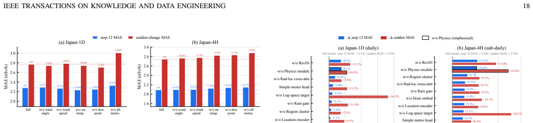
- [§V-A2, Fig. 8, Abstract] The sudden-change metric is defined as 'the top 10% of samples in the test set with the greatest variation between observed and predicted values' — i.e., per-model largest absolute residuals. This measures the right tail of each model's error distribution, not performance on genuine sudden changes in radiation. Different models have different worst-10% subsets, so the leaderboard in Fig. 8 compares incomparable denominators, and a model could rank first while being worse on true spikes. Please redefine the event set from ground-truth dynamics (e.g., observed increments exceeding a station-specific threshold) and re-report the sudden-change results. The issue is compounded by Appendix A-A, which shows that removing the log-space target changes 'sudden-change' MAE by +36.17% on Japan-1D, so the headline 19.1% gain may be largely attributable to preprocessing rather than to the physics modu
- [§III-C, §III-E, §III-F] Several descriptive analyses appear to use test-period or full-window information before the 60/20/20 split is applied. Fig. 3c explicitly reports Moran's I 'across the test period'; Fig. 4a and Fig. 6b are computed over the full dataset; and §III-F maps these findings directly to architectural components. If test-period statistics informed design choices, then the reported out-of-sample gains, including the 19.1% sudden-change improvement, are inflated. Please disclose the exact dates of the train/validation/test splits and rerun the key descriptive statistics (Moran's I, wind-stratified diffusion, stationarity tests) on the training portion only, or provide evidence that the design choices are insensitive to these statistics.
- [Table III vs Table II] The ablation table's full-model step-12 MAE values (2.0021 on Japan-4H and 2.2305 on Japan-1D) do not match the corresponding NRFormer+ 12-step MAE values in Table II (1.83 and 1.97). Since the ablation deltas are the basis for the claim that the physics module is one of the two largest contributors, the discrepancy must be reconciled. Please clarify the evaluation protocol for Table III (e.g., whether it is a single-step or recursive setting) and report the correct full-model baseline for each ablation row.
- [§IV-B1, Eqs. (5)-(6), Appendix A-A] The physics module's 'physics' content is largely a mean-deviation feature C_i^(P) − C̄^(P) plus a Softplus-constrained MLP that outputs D_i. The w/o Physics ablation removes both, so the reported +8–10% step-12 MAE degradation conflates removal of a generic global-anomaly feature with removal of a physics prior. Moreover, the learned D_i correlates positively with wind speed on Japan-4H but negatively on Japan-1D (Appendix A-A), and the paper does not resolve this inconsistency. Please run an ablation that removes only the Laplacian term and another that removes only D_i, and clarify what physical claim the learned coefficient actually supports.
minor comments (7)
- [§V-A2] The phrase 'greatest variation between observed and predicted values' should be stated as 'largest absolute error'; the current wording obscures that the metric is residual-based, not event-based.
- [Eq. (18)] The denormalization formula is missing parentheses: it should read ŷ_i = sqrt(Var[x_i]+ε) · (ỹ_i − β_i)/γ_i + E[x_i].
- [Fig. 1] The caption contains a stray token 'danwei' that should be removed.
- [§IV-B1] The statement that the advection term −u·∇C is 'absorbed by the density-adaptive spatial attention' is asserted rather than derived. Please justify or soften this claim.
- [Appendix A-A] The sign reversal of learned D_i versus wind speed between Japan-4H and Japan-1D is acknowledged but not resolved; at minimum, state a testable implication or a reason for the discrepancy.
- [Table III] The heading 'single-step metrics at the 12th forecasting horizon' is confusing and should be clarified relative to the multi-step results in Table II.
- [§V-A4] The exact dates of the 60/20/20 split are not disclosed. Please provide them, as this is essential for evaluating the independence of the Section III analyses.
Circularity Check
Two evaluation-side circularities: 'sudden-change' is defined on the model's own residuals, and the motivating data analysis explicitly used the test period; core learned modules are otherwise not circular.
-
self definitional
[Section V-A2 (Evaluation Metrics); abstract and Section V-B conclusions]
"We identified the top 10% of samples in the test set with the greatest variation between observed and predicted values as sudden-change samples for prediction."
The 'sudden-change' subset is defined as each model's largest absolute residuals, so 'sudden-change MAE' is a tail statistic of the model's own error distribution. The abstract's 'reducing sudden-change MAE by up to 19.1%' and Section V-C's conclusion that NRFormer+ 'adapts more quickly to the non-stationary nature of radiation' therefore measure residual-tail behavior, not genuine sudden-change events. Because the subset is re-derived per model, the comparison has different denominators and the headline gain is an artifact of the metric definition.
-
fitted input called prediction
[Section III-C, III-E, III-F; Figure 3(c)]
"Time-averaged global Moran's I=0.15 on radiation residuals across the test period. ... This directly motivates the Density-Adaptive Spatial Attention ... the resulting empirical signatures ... collectively define the design space within which NRFormer+ operates."
The data analyses that motivate the model components (spatial attention, wind-modulated diffusion, seasonal embedding) are computed on the full corpus, explicitly including the test period. Those same components are then evaluated on the test period. The 'out-of-sample' claim is thus partly in-sample: the test period has already informed which inductive biases to use, so the reported gains, including the 19.1% sudden-change improvement, are not a clean prediction of an unseen period.
full rationale
The core forecasting pipeline is not mathematically circular: the diffusion coefficient in Eq. (5) is learned from training data, the mean-field Laplacian in Eq. (6) is a parameter-free feature, and the ablation study independently evaluates each component. Self-citation of NRFormer [24] is used only as a baseline and starting point, not to establish a uniqueness theorem or to forbid alternatives. No equation in the model reduces to its inputs by construction. However, two evaluation-side steps are circular. First, the 'sudden-change MAE' metric defines sudden-change samples as the top 10% of residuals between observed and predicted values, so the metric is self-referential: it measures the tail of each model's own error distribution rather than physical sudden changes, and the headline 19.1% improvement is an artifact of that definition. Second, the motivating data analysis explicitly includes the test period (Figure 3(c)) and Section III-F states that the resulting findings 'collectively define the design space' for the architecture; evaluating on that same test period means the architecture selection was informed by the evaluation set. These issues do not invalidate the independent overall-MAE results, but they make the paper's flagship sudden-change claim and its strict out-of-sample claim partially circular.
Assumptions & free parameters
free parameters (4)
- L_t (temporal attention depth) =
4 (Japan-1D), 3 (Japan-4H)
- L_s (spatial attention depth) =
2 (both datasets)
- Distance threshold for adjacency matrix A =
not reported
- Hidden dimension D =
not reported
assumptions (4)
- domain assumption Advection–diffusion PDE (Eq. 4) governs radionuclide transport
- ad hoc to paper ∇²C_i ≈ C_i − C̄ (mean-field Laplacian surrogate)
- ad hoc to paper Density-adaptive spatial attention absorbs the advection term −u·∇C
- domain assumption Meteorological variables from 228 NOAA stations, interpolated to 3,627 radiation sites, are representative of local conditions
Cite this review
Pith. "Pith review of Atmospheric Diffusion-Guided Spatio-Temporal Transformer for Nuclear Radiation Forecasting." pith.science (2026). https://pith.science/paper/US7X72FF
@misc{pith2026260724774,
  author       = {Pith},
  title        = {Pith review of: Atmospheric Diffusion-Guided Spatio-Temporal Transformer for Nuclear Radiation Forecasting},
  year         = {2026},
  howpublished = {\url{https://pith.science/paper/US7X72FF}},
  note         = {Machine review of arXiv:2607.24774}
}
read the original abstract
Nuclear radiation, the energy released during atomic decay, poses persistent risks to public health and the environment, and concerns have only grown since the Fukushima accident and the recent commencement of treated-water discharge. Modern monitoring networks now record radiation levels and accompanying weather conditions at thousands of stations, opening the door to nationwide forecasting that can inform emergency response, agricultural advisories, and routine public-safety decisions. However, turning this abundance of monitoring data into reliable forecasts is difficult for three reasons. First, the time series at each station are highly non-stationary, shaped by radioactive decay, weather variability, and irregular human interventions. Second, monitoring stations are severely unevenly distributed in space. Roughly 78% of Japan's stations sit in less than 6% of the country, clustered near Fukushima, which breaks the assumptions of standard graph-based models. Third, radiation co-evolves with heterogeneous context such as wind, temperature, and humidity through atmospheric transport processes that purely data-driven models struggle to capture from observations alone. In this study, we introduce NRFormer+, a spatio-temporal Transformer for nationwide nuclear radiation forecasting. NRFormer+ couples non-stationary temporal attention and density-adaptive spatial attention with a new atmospheric diffusion module that estimates how meteorology drives radiation dispersion and injects this physical signal into the network as an architectural prior. NRFormer+ delivers state-of-the-art accuracy on both datasets across all 13 baselines, reducing sudden-change MAE by up to 19.1% over the strongest baseline at comparable inference latency. Our code and datasets are publicly available at https://github.com/tfeilyu/NRFormer_Plus.
Figures


Figures from the paper (9 more)




Reference graph
Works this paper leans on
-
[1]
The wildfire problem in areas contaminated by the chernobyl disaster,
A. A. Ager, R. Lasko, V . Myroniuk, S. Zibtsev, M. A. Day, U. Usenia, V . Bogomolov, I. Kovalets, and C. R. Evers, “The wildfire problem in areas contaminated by the chernobyl disaster,”Science of the Total Environment, vol. 696, p. 133954, 2019
2019
-
[2]
Comparison of the cher- nobyl and fukushima nuclear accidents: a review of the environmental impacts,
G. Steinhauser, A. Brandl, and T. E. Johnson, “Comparison of the cher- nobyl and fukushima nuclear accidents: a review of the environmental impacts,”Science of the total environment, vol. 470, pp. 800–817, 2014
2014
-
[3]
Predicting the spread of nuclear radiation from the damaged fukushima nuclear power plant,
F. Qiao, G. Wang, W. Zhao, J. Zhao, D. Dai, Y . Song, and Z. Song, “Predicting the spread of nuclear radiation from the damaged fukushima nuclear power plant,”Chinese Science Bulletin, vol. 56, pp. 1890–1896, 2011
2011
-
[4]
The mathematics of atmospheric dispersion modeling,
J. M. Stockie, “The mathematics of atmospheric dispersion modeling,” SIAM Review, vol. 53, no. 2, pp. 349–372, 2011
2011
-
[5]
Noaa’s HYSPLIT atmospheric transport and dispersion modeling system,
A. Stein, R. R. Draxler, G. D. Rolph, B. J. Stunder, M. Cohen, and F. Ngan, “Noaa’s HYSPLIT atmospheric transport and dispersion modeling system,”Bulletin of the American Meteorological Society, vol. 96, no. 12, pp. 2059–2077, 2015
-
[6]
Technical note: The lagrangian particle dispersion model FLEXPART version 6.2,
A. Stohl, C. Forster, A. Frank, P. Seibert, and G. Wotawa, “Technical note: The lagrangian particle dispersion model FLEXPART version 6.2,” Atmospheric Chemistry and Physics, vol. 5, no. 9, pp. 2461–2474, 2005
2005
-
[7]
Xenon-133 and caesium-137 releases into the atmosphere from the Fukushima Dai-ichi nuclear power plant: determination of the source term, atmospheric dispersion, and deposition,
A. Stohl, P. Seibert, G. Wotawa, D. Arnold, J. F. Burkhart, S. Eckhardt, C. Tapia, A. Vargas, and T. J. Yasunari, “Xenon-133 and caesium-137 releases into the atmosphere from the Fukushima Dai-ichi nuclear power plant: determination of the source term, atmospheric dispersion, and deposition,”Atmospheric Chemistry and Physics, vol. 12, pp. 2313– 2343, 2012
2012
-
[8]
Graph wavenet for deep spatial-temporal graph modeling,
Z. Wu, S. Pan, G. Long, J. Jiang, and C. Zhang, “Graph wavenet for deep spatial-temporal graph modeling,”arXiv preprint arXiv:1906.00121, 2019
arXiv 1906
Show all 47 references
-
[9]
AutoCTS: Automated correlated time series forecasting,
X. Wu, D. Zhang, C. Guo, C. He, B. Yang, and C. S. Jensen, “AutoCTS: Automated correlated time series forecasting,”Proceedings of the VLDB Endowment, vol. 15, no. 4, pp. 971–983, 2022
2022
-
[10]
Bigst: Linear complexity spatio-temporal graph neural network for traffic forecasting on large-scale road networks,
J. Han, W. Zhang, H. Liu, T. Tao, N. Tan, and H. Xiong, “Bigst: Linear complexity spatio-temporal graph neural network for traffic forecasting on large-scale road networks,”Proceedings of the VLDB Endowment, vol. 17, no. 5, pp. 1081–1090, 2024
2024
-
[11]
Informer: Beyond efficient transformer for long sequence time-series forecasting,
H. Zhou, S. Zhang, J. Peng, S. Zhang, J. Li, H. Xiong, and W. Zhang, “Informer: Beyond efficient transformer for long sequence time-series forecasting,” inProceedings of the AAAI conference on artificial intel- ligence, vol. 35, no. 12, 2021, pp. 11 106–11 115
2021
-
[12]
iTrans- former: Inverted transformers are effective for time series forecasting,
Y . Liu, T. Hu, H. Zhang, H. Wu, S. Wang, L. Ma, and M. Long, “iTrans- former: Inverted transformers are effective for time series forecasting,” inInternational Conference on Learning Representations, 2024
2024
-
[13]
Koopa: Learning non-stationary time series dynamics with koopman predictors,
Y . Liu, C. Li, J. Wang, and M. Long, “Koopa: Learning non-stationary time series dynamics with koopman predictors,”Advances in Neural Information Processing Systems, vol. 36, 2024
2024
-
[14]
Airformer: Predicting nationwide air quality in china with transformers,
Y . Liang, Y . Xia, S. Ke, Y . Wang, Q. Wen, J. Zhang, Y . Zheng, and R. Zimmermann, “Airformer: Predicting nationwide air quality in china with transformers,” inProceedings of the AAAI Conference on Artificial Intelligence, vol. 37, no. 12, 2023, pp. 14 329–14 337
2023
-
[15]
AirPhyNet: Harnessing physics-guided neural networks for air qual- ity prediction,
K. H. Hettige, J. Ji, S. Xiang, C. Long, G. Cong, and J. Wang, “AirPhyNet: Harnessing physics-guided neural networks for air qual- ity prediction,” inThe Twelfth International Conference on Learning Representations (ICLR), 2024. IEEE TRANSACTIONS ON KNOWLEDGE AND DATA ENGINEERING 14
2024
-
[16]
TFB: Towards comprehensive and fair benchmarking of time series forecasting methods,
X. Qiu, J. Hu, L. Zhou, X. Wu, J. Du, B. Zhang, C. Guo, A. Zhou, C. S. Jensen, Z. Sheng, and B. Yang, “TFB: Towards comprehensive and fair benchmarking of time series forecasting methods,”Proceedings of the VLDB Endowment, vol. 17, no. 9, pp. 2363–2377, 2024
2024
-
[17]
Reversible instance normalization for accurate time-series forecasting against distri- bution shift,
T. Kim, J. Kim, Y . Tae, C. Park, J.-H. Choi, and J. Choo, “Reversible instance normalization for accurate time-series forecasting against distri- bution shift,” inInternational Conference on Learning Representations, 2021
2021
-
[18]
Non-stationary transformers: Exploring the stationarity in time series forecasting,
Y . Liu, H. Wu, J. Wang, and M. Long, “Non-stationary transformers: Exploring the stationarity in time series forecasting,”Advances in Neural Information Processing Systems, vol. 35, pp. 9881–9893, 2022
2022
-
[19]
Physics-informed neural networks: A deep learning framework for solving forward and inverse problems involving nonlinear partial differential equations,
M. Raissi, P. Perdikaris, and G. E. Karniadakis, “Physics-informed neural networks: A deep learning framework for solving forward and inverse problems involving nonlinear partial differential equations,” Journal of Computational Physics, vol. 378, pp. 686–707, 2019
2019
-
[20]
Hidden fluid mechanics: Learning velocity and pressure fields from flow visualizations,
M. Raissi, A. Yazdani, and G. E. Karniadakis, “Hidden fluid mechanics: Learning velocity and pressure fields from flow visualizations,”Science, vol. 367, no. 6481, pp. 1026–1030, 2020
2020
-
[21]
Enforcing analytic constraints in neural networks emulating physical systems,
T. Beucler, M. Pritchard, S. Rasp, J. Ott, P. Baldi, and P. Gentine, “Enforcing analytic constraints in neural networks emulating physical systems,”Physical Review Letters, vol. 126, no. 9, p. 098302, 2021
2021
-
[22]
Learning skillful medium-range global weather forecasting,
R. Lam, A. Sanchez-Gonzalez, M. Willson, P. Wirnsberger, M. For- tunato, F. Alet, S. Ravuri, T. Ewalds, Z. Eaton-Rosen, W. Huet al., “Learning skillful medium-range global weather forecasting,”Science, vol. 382, no. 6677, pp. 1416–1421, 2023
2023
-
[23]
FourCastNet: A global data-driven high-resolution weather forecasting model,
J. Pathak, S. Subramanian, P. Harrington, S. Raja, A. Chattopadhyay, M. Mardani, T. Kurth, D. Hall, Z. Li, K. Azizzadenesheliet al., “FourCastNet: A global data-driven high-resolution weather forecasting model,” inProceedings of the Platform for Advanced Scientific Com- puting...
2022
-
[24]
Nrformer: Nationwide nuclear radiation forecasting with spatio-temporal transformer,
T. Lyu, J. Han, and H. Liu, “Nrformer: Nationwide nuclear radiation forecasting with spatio-temporal transformer,” inProceedings of the 31st ACM SIGKDD Conference on Knowledge Discovery and Data Mining, 2025
2025
-
[25]
Distribution of the estimators for autoregressive time series with a unit root,
D. A. Dickey and W. A. Fuller, “Distribution of the estimators for autoregressive time series with a unit root,”Journal of the American Statistical Association, vol. 74, no. 366a, pp. 427–431, 1979
1979
-
[26]
Testing the null hypothesis of stationarity against the alternative of a unit root: How sure are we that economic time series have a unit root?
D. Kwiatkowski, P. C. B. Phillips, P. Schmidt, and Y . Shin, “Testing the null hypothesis of stationarity against the alternative of a unit root: How sure are we that economic time series have a unit root?”Journal of Econometrics, vol. 54, no. 1-3, pp. 159–178, 1992
1992
-
[27]
Attention is all you need,
A. Vaswani, N. Shazeer, N. Parmar, J. Uszkoreit, L. Jones, A. N. Gomez, Ł. Kaiser, and I. Polosukhin, “Attention is all you need,”Advances in neural information processing systems, vol. 30, 2017
2017
-
[28]
The emerging field of signal processing on graphs: Ex- tending high-dimensional data analysis to networks and other irregular domains,
D. I. Shuman, S. K. Narang, P. Frossard, A. Ortega, and P. Van- dergheynst, “The emerging field of signal processing on graphs: Ex- tending high-dimensional data analysis to networks and other irregular domains,”IEEE Signal Processing Magazine, vol. 30, no. 3, pp. 83–98, 2013
2013
-
[29]
Forecasting fine-grained air quality based on big data,
Y . Zheng, X. Yi, M. Li, R. Li, Z. Shan, E. Chang, and T. Li, “Forecasting fine-grained air quality based on big data,” inProceedings of the 21th ACM SIGKDD international conference on knowledge discovery and data mining, 2015, pp. 2267–2276
2015
-
[30]
Deep distributed fusion network for air quality prediction,
X. Yi, J. Zhang, Z. Wang, T. Li, and Y . Zheng, “Deep distributed fusion network for air quality prediction,” inProceedings of the 24th ACM SIGKDD international conference on knowledge discovery & data mining, 2018, pp. 965–973
2018
-
[31]
Decoupled dynamic spatial-temporal graph neural network for traffic forecasting,
Z. Shao, Z. Zhang, W. Wei, F. Wang, Y . Xu, X. Cao, and C. S. Jensen, “Decoupled dynamic spatial-temporal graph neural network for traffic forecasting,”Proceedings of the VLDB Endowment, vol. 15, no. 11, pp. 2733–2746, 2022
2022
-
[32]
Xgboost: A scalable tree boosting system,
T. Chen and C. Guestrin, “Xgboost: A scalable tree boosting system,” inProceedings of the 22nd ACM SIGKDD International Conference on Knowledge Discovery and Data Mining, 2016, pp. 785–794
2016
-
[33]
Diffusion convolutional recurrent neural network: Data-driven traffic forecasting,
Y . Li, R. Yu, C. Shahabi, and Y . Liu, “Diffusion convolutional recurrent neural network: Data-driven traffic forecasting,” inInternational Con- ference on Learning Representations, 2018
2018
-
[34]
Spectral temporal graph neural network for multivariate time-series forecasting,
D. Cao, Y . Wang, J. Duan, C. Zhang, X. Zhu, C. Huang, Y . Tong, B. Xu, J. Bai, J. Tonget al., “Spectral temporal graph neural network for multivariate time-series forecasting,”Advances in neural information processing systems, vol. 33, pp. 17 766–17 778, 2020
2020
-
[35]
Spatial-temporal identity: A simple yet effective baseline for multivariate time series forecasting,
Z. Shao, Z. Zhang, F. Wang, W. Wei, and Y . Xu, “Spatial-temporal identity: A simple yet effective baseline for multivariate time series forecasting,” inProceedings of the 31st ACM International Conference on Information and Knowledge Management, 2022, pp. 4454–4458
2022
-
[36]
Lightcts: A lightweight framework for correlated time series forecasting,
Z. Lai, D. Zhang, H. Li, C. S. Jensen, H. Lu, and Y . Zhao, “Lightcts: A lightweight framework for correlated time series forecasting,”Pro- ceedings of the ACM on Management of Data, vol. 1, no. 2, pp. 1–26, 2023
2023
-
[37]
Are transformers effective for time series forecasting?
A. Zeng, M. Chen, L. Zhang, and Q. Xu, “Are transformers effective for time series forecasting?” inProceedings of the AAAI conference on artificial intelligence, vol. 37, no. 9, 2023, pp. 11 121–11 128
2023
-
[38]
A time series is worth 64 words: Long-term forecasting with transformers,
Y . Nie, N. H. Nguyen, P. Sinthong, and J. Kalagnanam, “A time series is worth 64 words: Long-term forecasting with transformers,” inThe Eleventh International Conference on Learning Representations, 2023
2023
-
[39]
Timesnet: Temporal 2d-variation modeling for general time series analysis,
H. Wu, T. Hu, Y . Liu, H. Zhou, J. Wang, and M. Long, “Timesnet: Temporal 2d-variation modeling for general time series analysis,” inThe Eleventh International Conference on Learning Representations, 2022
2022
-
[40]
Spatio-temporal graph neural networks for predictive learning in urban computing: A survey,
G. Jin, Y . Liang, Y . Fang, Z. Shao, J. Huang, J. Zhang, and Y . Zheng, “Spatio-temporal graph neural networks for predictive learning in urban computing: A survey,”IEEE Transactions on Knowledge and Data Engineering, 2023
2023
-
[41]
Towards spatio- temporal aware traffic time series forecasting,
R.-G. Cirstea, B. Yang, C. Guo, T. Kieu, and S. Pan, “Towards spatio- temporal aware traffic time series forecasting,” in2022 IEEE 38th International Conference on Data Engineering (ICDE). IEEE, 2022, pp. 2900–2913
2022
-
[42]
Fourier neural operator for parametric partial differential equations,
Z. Li, N. Kovachki, K. Azizzadenesheli, B. Liu, K. Bhatt, A. Stuart, and A. Anandkumar, “Fourier neural operator for parametric partial differential equations,”arXiv preprint arXiv:2010.08895, 2021
2010 arXiv
-
[43]
Deep learning for spatio-temporal data mining: A survey,
S. Wang, J. Cao, and P. S. Yu, “Deep learning for spatio-temporal data mining: A survey,”IEEE Transactions on Knowledge and Data Engineering, vol. 34, no. 8, pp. 3681–3700, 2022
2022
-
[44]
The RODOS system: Decision support for off-site emergency management in Europe,
J. Ehrhardt and A. Weis, “The RODOS system: Decision support for off-site emergency management in Europe,”Radiation Protection Dosimetry, vol. 91, no. 1-3, pp. 291–295, 2000
2000
-
[45]
Winiarek, M
V . Winiarek, M. Bocquet, O. Saunier, and A. Mathieu, “Estimation of errors in the inverse modeling of accidental release of atmospheric pollutant: Application to the reconstruction of the cesium-137 and iodine-131 source terms from the Fukushima Daiichi power plant,” Journal ...
2012
-
[46]
Spatial and temporal prediction of radiation dose rates near fukushima daiichi nuclear power plant,
D. Sun, H. Wainwright, I. Suresh, A. Seki, H. Takemiya, and K. Saito, “Spatial and temporal prediction of radiation dose rates near fukushima daiichi nuclear power plant,”Journal of Environmental Radioactivity, vol. 251, p. 106946, 2022. Tengfei Lyuis a PhD student at the Thru...
2022
-
[2025]
He have published over 30 papers in prestigious journals and confer- ences, such as IEEE TKDE, KDD, WWW, VLDB, NeurIPS, ICLR, and AAAI
His research focuses on data mining, urban intelligence, and AI for science. He have published over 30 papers in prestigious journals and confer- ences, such as IEEE TKDE, KDD, WWW, VLDB, NeurIPS, ICLR, and AAAI. Hao Liureceived the BE degree from the South China University of...
2012
Reviewed August 2, 2026 · model on record in the stance chip above.
Discussion (0). Sign in to comment.