REVIEW 2 major objections 6 minor 67 references
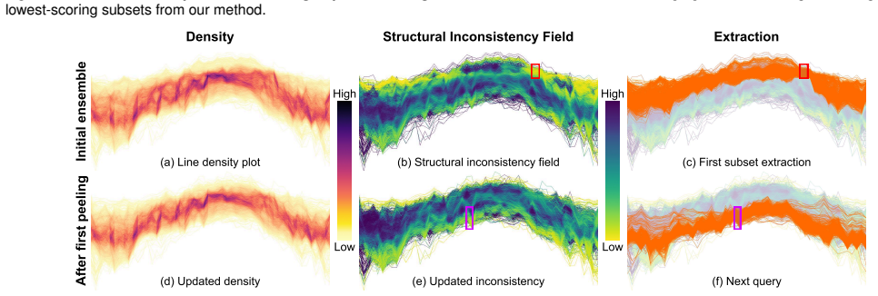
Dense line plots hide whether trajectories agree; a path-integrated fidelity score and Structural Inconsistency Field expose where clutter is coherent and where it breaks.
Reviewed by Pith at T0; open to challenge. T0 means a machine referee read the full paper against a public rubric. the ladder, T0–T4 →
T0 review · grok-4.5
2026-07-31 00:40 UTC pith:LV74AWPE
load-bearing objection Solid, usable viz method: density’s missing “agreement” channel via tensor path integrals and SIF, with real limits on ℓ and majority orientation that the paper mostly owns. the 2 major comments →
Structuring Line Ensembles with Path-Integrated Fidelity and Structural Inconsistency Fields
The pith
A machine-rendered reading of the paper's core claim, the machinery that carries it, and where it could break.
Core claim
When paired with ordinary density views, path-integrated trajectory fidelity against an ensemble structure-tensor field—corrected by dynamic leave-one-out and reprojected as a passage-centered Structural Inconsistency Field—disambiguates dense line patterns by localizing sustained structural support versus disagreement, outliers, and connectivity-induced ambiguity that scalar accumulation cannot separate.
What carries the argument
Structural Inconsistency Field (SIF): one minus the mean leave-one-out, path-extent-averaged orientation support of every trajectory passage through a pixel, so low values mark coherent support and high values mark conflict or weak evidence.
Load-bearing premise
The method treats agreement with the majority’s undirected local orientation, after removing the line itself and integrating over a chosen path length, as enough to call a dense pattern structurally supported—even in flat crossings and in 2D views of 3D fibers.
What would settle it
On controlled ensembles like the paper’s D1–D3 (hidden cuts, lane changes, connected vs disconnected bridges), check whether SIF-based line scores still separate ground-truth outliers or connectivity better than density (AUROC/AUPRC) when path extent is wrong, leave-one-out is off, or the majority orientation is adversarial or antiparallel counterflow that must be distinguished.
If this is right
- Density maps can be read jointly with SIF so analysts query coherent corridors instead of hotspots that mix incompatible paths.
- Trajectory-fidelity ranking enables iterative peeling: remove high- or low-support subsets and recompute to expose secondary structure under dominant clutter.
- Fixed-grid tensor construction plus prefix-sum path extents keep the pipeline interactive for tens of thousands of lines in browser-side settings.
- Screen-space scoring can recover readable projected scaffolds from fiber or traffic data without deforming geometry the way bundling does.
- Sparse one- or two-line neighborhoods after leave-one-out should be read with density or passage count as low-confidence evidence, not automatic conflict.
Where Pith is reading between the lines
- Any domain that already ships density or occupancy heatmaps of paths (mobility, climate series, tractography) could add SIF as a second channel without replacing existing overview tools.
- Direction-aware tensors (not only undirected outer products) would be a direct next test wherever opposing flows must not reinforce each other.
- Coupling SIF confidence with passage count could turn “high inconsistency” versus “insufficient evidence” into an explicit visual layer the current mask does not separate.
Editorial analysis
A structured set of objections, weighed in public.
Referee Report
Summary. The paper proposes a tensor-guided, path-integrated fidelity measure for large line ensembles: each grid cell accumulates a structure tensor from rasterized trajectory tangents, each trajectory is scored against this field via a trace-normalized quadratic form with dynamic leave-one-out correction, and passage-centered averages of this score are projected back into image space as a Structural Inconsistency Field (SIF, Eq. 6). The SIF is meant to complement scalar density by distinguishing coherent bundles from conflict, outliers, and connectivity ambiguity. The paper evaluates on three synthetic benchmarks (D1–D3) with line-level AUROC/AUPRC against a density baseline (Table 1), a scalability study against a Hausdorff reference (Fig. 10), a controlled LOO ablation on nested spindle ensembles (Table 2, App. E), and several real-world case studies (ACIS temperatures, France aviation, DTI fibers, plus four more in App. F). The central claim is that, paired with density views, the SIF exposes spatially localized coherence and structural breakdown that density-only representations conceal.
Significance. If the results hold, this is a useful, practical addition to the line-ensemble visualization toolbox. Strengths worth naming: (1) the construction is fully explicit and parameter-light at its core — the structure tensor is a strict extension of density (tr(J)=D), the LOO score has a clean counterfactual interpretation, and the SIF is bounded in [0,1]; (2) the LOO ablation (Table 2) is a genuinely controlled experiment with bootstrap confidence intervals showing that without LOO the ranking inverts (AUROC 0.009 vs 0.831), which substantiates the self-bias argument rather than merely asserting it; (3) quantitative line-level separation on D1/D2 is reported with appropriate imbalanced-class metrics (AUPRC alongside AUROC); (4) the method scales to browser-side interactive use via fixed-grid accumulation and prefix sums, avoiding the O(N²) wall of pairwise-distance methods; (5) an interactive online system is referenced, supporting reproducibility. The limitations (majority-rules logic, undirected orientation, isotropic ambiguity, view-dependence) are acknowledged honestly. The significance is narrowed mainly by the fact that 'structural support' is majority-orientation support over a
major comments (2)
- [§5.1, Table 1; App. D, Fig. 24] The headline quantitative result reports AUROC/AUPRC for D1 at path extent ℓ=1 and D2 at ℓ=150, i.e., the path-extent parameter appears to be tuned per dataset. Appendix D demonstrates qualitatively (Fig. 24) that D3-C/D3-D separate only at maximal extent, so the metric's discriminative power is demonstrably ℓ-dependent, yet no sensitivity sweep (AUROC/AUPRC vs. ℓ), no selection rule, and no resolution-invariant normalization of ℓ is provided for the quantitative benchmarks. Appendix D also states that the discrete ℓ values 'depend on the discretization resolution' and must be re-chosen when resolution changes. Since Table 1 is the only quantitative evidence that the SIF separates outliers from inliers, the authors should (i) report the AUROC/AUPRC curves over a range of ℓ for D1 and D2, and (ii) give practical guidance on ℓ selection (e.g., relative to bundle length or grid resolution).
- [§4.2–4.4; §6 (Limitations); Abstract] The definitions of support (Eqs. 4, 5, 6, 14) score agreement with the majority-orientation structure tensor. The paper is commendably explicit about the consequences (majority-rules logic, undirected vvᵀ accumulation so antiparallel counterflow reinforces rather than conflicts, E≈0.5 ambiguity in isotropic regions, view-dependence of 2D projections of 3D fibers; §6 and App. F.3.1). However, the Abstract and Conclusion phrase the outcome as exposing 'spatially localized coherence and structural breakdown' without the qualifier that this is majority-orientation support under a user-chosen extent. Since App. F.3.1 itself shows a valid minority structure (the 370-line late-starting stock subset) being marked highly inconsistent by the field, the framing in the Abstract/Conclusion should be tightened to match what the metric actually measures, so that readers do not over-read the real-data c
minor comments (6)
- [§5.1, Table 1] Table 1, D1 row: the SIF AUPRC of 0.3679 is much better than density (0.0089) but modest in absolute terms given ~1% prevalence. A sentence contextualizing this value (e.g., precision at a fixed recall) would help readers calibrate the claim.
- [§4.4, App. B] The symbol ℓ is used both as a continuous arc length (Eq. 13–14) and as a count of rasterized samples in the discrete implementation ('we keep the same symbol ℓ'). Since the two scale differently with grid resolution, consider distinct notation or an explicit conversion; this is also the root of the resolution-dependence noted in App. D.
- [§4.2] The matched-filter analogy is evocative but imprecise: a matched filter maximizes SNR against a known template, whereas here the 'template' (tensor field) is itself estimated from the ensemble and modified per query by LOO. A brief qualifier would avoid over-reading.
- [§5.2, Fig. 10] Timings are single runs on one browser/machine with acknowledged JIT/GC variability. Even a small number of repetitions with min/median reporting would strengthen the scalability claim, particularly the '~2.4 s at N=10,000' headline.
- [§4.2, Eq. (4)] It would help to state the value of ε (and its effect) used in the main-text experiments, as it is only specified in the App. E ablation (ε=0 with the zero-support convention). Similarly, kernel bandwidth σ and grid resolution per experiment should be collected in one place for reproducibility.
- [Fig. 1] Fig. 1 axis label shows '120 °F' without units context in the caption; caption should state that values are weekly maxima in °F over the year axis. Minor figure-clarity issue.
Circularity Check
No significant circularity: SIF/fidelity are constructive functionals validated against external labels, not self-fulfilling predictions.
full rationale
The paper defines a structure tensor from the ensemble, a leave-one-out path-integrated fidelity Φ(L), and a passage-centered Structural Inconsistency Field M(x;ℓ)=1−mean φ, then evaluates these scores on synthetic tasks with independent ground-truth classes (D1/D2 AUROC/AUPRC vs density) and qualitative real-world cases. That pipeline is definitional engineering of a metric, not a claim that a fitted free parameter predicts a quantity forced by the fit. Self-citations to Xue et al. on density illumination and image-space colorization are used as perceptual/baseline comparisons, not as uniqueness theorems or load-bearing premises that force the present result. LOO is a counterfactual correction against self-support, not circular reuse of the target. Boundary conditions (majority-rules, undirected vvT, ℓ sensitivity) are limitations of the operational definition, not circular reductions of claim to input. No fitted-input-called-prediction or self-definitional X⇔Y step appears in the derivation chain.
Axiom & Free-Parameter Ledger
free parameters (5)
- path extent ℓ =
task-dependent (examples: 1; 150; 0/400/1000 on D3)
- spatial kernel bandwidth h / Gaussian σ and kernel support =
implementation/grid dependent
- analysis grid resolution =
e.g. 1000×500 (perf); other canvases in appendix
- density regularization ε =
ε small or 0 with explicit zero-support rule
- peel / rank percentiles and query windows =
case-specific (80/20, 50/50, 3/97, etc.)
axioms (6)
- domain assumption Second-moment structure tensors from tangent outer products are an adequate local summary of orientation mass without sign cancellation.
- ad hoc to paper Structural support means agreement of a trajectory tangent with the leave-one-out ensemble tensor along a path, not geometric centrality or pairwise distance.
- domain assumption Undirected orientation (vvT) is acceptable, so antiparallel traffic reinforces rather than cancels.
- domain assumption Fixed-grid 2D screen-space binning (including orthographic projections of 3D fibers) is a valid analysis domain for the claimed interactive structuring.
- standard math Curve density / kernel splatting on a raster is a faithful enough discrete stand-in for continuous occupancy and tensor mass.
- ad hoc to paper After LOO, absence of remaining tensor mass should score as zero independent support rather than undefined or self-supported agreement.
invented entities (3)
-
Structural Inconsistency Field (SIF) M(x;ℓ)
independent evidence
-
Path-integrated trajectory fidelity Φ(L) with dynamic LOO
independent evidence
-
Passage-centered support φ(L,sx;ℓ)
independent evidence
read the original abstract
When visualizing large-scale line ensembles, trajectory continuity and visual scalability are inherently antagonistic. Trajectory-centric renderings preserve path information but rapidly degenerate into clutter as line density increases and mutual occlusion dominates. In contrast, field-based density representations enhance visibility while sacrificing structural coherence: density reflects accumulation rather than agreement, such that scalar aggregation alone cannot discriminate between consistent and conflicting configurations. Rather than replacing density-based views, we complement them with a path-integrated trajectory-fidelity measure that quantifies the agreement of each trajectory with a surrounding tensor field. By projecting this passage-centered structural support back into image space, we obtain what we call a Structural Inconsistency Field, which localizes regions where dense patterns correspond to coherent structure versus disagreement, outliers, or connectivity-induced ambiguity. Dynamic leave-one-out correction reduces self-bias in the path integral. Efficient fixed-grid updates combined with prefix-sum evaluation enable interactive analysis and iterative extraction of coherent structures. Synthetic benchmarks, scalability analyses, and real-world case studies demonstrate that, when paired with conventional density views, the proposed method disambiguates dense line patterns by exposing spatially localized coherence and structural breakdown that remain concealed in density-only representations.
Figures






Reference graph
Works this paper leans on
-
[1]
Akmal Butt and P
M. Akmal Butt and P. Maragos. Optimum design of chamfer distance transforms.IEEE Transactions on Image Processing, 7(10):1477–1484,
-
[2]
ACIS web services.http://www
Applied Climate Information System. ACIS web services.http://www. rcc-acis.org/docs_webservices.html, 2017. Accessed: 2026-06-
2017
-
[3]
Hard drive data and stats
Backblaze. Hard drive data and stats. https://www.backblaze.com/ b2/hard-drive-test-data.html, 2013. Accessed: 2026-06-15. 15
2013
-
[4]
J. Bian, D. Tian, Y . Tang, and D. Tao. A survey on trajectory clustering analysis.arXiv preprint, 2018. doi: 10.48550/arXiv.1802.06971 2
-
[5]
A. W. Bowman. An alternative method of cross-validation for the smooth- ing of density estimates.Biometrika, 71(2):353–360, 1984. doi: 10. 1093/biomet/71.2.353 5
1984
-
[6]
A. Brambilla, R. Carnecky, R. Peikert, I. Viola, and H. Hauser. Illustrative flow visualization: State of the art, trends and challenges. In M.-P. Cani and F. Ganovelli, eds.,Eurographics 2012 - State of the Art Reports. The Eurographics Association, 2012. doi: 10.2312/conf/EG2012/stars/075-094 1
-
[7]
K. J. Burns, G. M. Vasil, J. S. Oishi, D. Lecoanet, and B. P. Brown. Dedalus: A flexible framework for numerical simulations with spectral methods.Physical Review Research, 2(2):023068, 2020. doi: 10.1103/ PhysRevResearch.2.023068 14
2020
-
[8]
B. Cabral and L. C. Leedom. Imaging vector fields using line integral convolution. InProceedings of the 20th Annual Conference on Computer Graphics and Interactive Techniques, SIGGRAPH ’93, pp. 263–270. ACM, New York, 1993. doi: 10.1145/166117.166151 2, 3
arXiv 1993
-
[10]
W. Chen, F. Guo, and F.-Y . Wang. A survey of traffic data visualization. IEEE Transactions on Intelligent Transportation Systems, 16(6):2970– 2984, 2015. doi: 10.1109/TITS.2015.2436897 1, 2
arXiv 2015
-
[11]
X. Chen, Y . Wang, H. Bao, K. Lu, J. Jo, C.-W. Fu et al. Visualization- driven illumination for density plots.IEEE Transactions on Visualization and Computer Graphics, 31(2):1631–1644, 2025. doi: 10.1109/TVCG. 2024.3495695 3
arXiv 2025
-
[12]
U. Diewald, T. Preusser, and M. Rumpf. Anisotropic diffusion in vector field visualization on Euclidean domains and surfaces.IEEE Transactions on Visualization and Computer Graphics, 6(2):139–149, 2000. doi: 10. 1109/2945.856995 2
arXiv 2000
-
[13]
Eichelbaum, M
S. Eichelbaum, M. Hlawitschka, and G. Scheuermann. Lin- eAO—improved three-dimensional line rendering.IEEE Transactions on Visualization and Computer Graphics, 19(3):433–445, 2013. doi: 10. 1109/TVCG.2012.142 3
2013
-
[14]
M. H. Everts, E. Begue, H. Bekker, J. B. T. M. Roerdink, and T. Isen- berg. Exploration of the brain’s white matter structure through visual abstraction and multi-scale local fiber tract contraction.IEEE Transac- tions on Visualization and Computer Graphics, 21(7):808–821, 2015. doi: 10.1109/TVCG.2015.2403323 8
arXiv 2015
-
[15]
T. Fawcett. An introduction to ROC analysis.Pattern Recognition Letters, 27(8):861–874, 2006. doi: 10.1016/j.patrec.2005.10.010 7
-
[16]
A. Frantzis, R. Leaper, P. Alexiadou, A. Prospathopoulos, and D. Lekkas. Hellenic Trench AIS data, 2018. doi: 10.17882/57040 15
-
[17]
T. Günther, C. Rössl, and H. Theisel. Opacity optimization for 3D line fields.ACM Trans. Graph., 32(4), art. no. 120, 8 pp., July 2013. doi: 10. 1145/2461912.2461930 3
arXiv 2013
-
[18]
H. Guo, W. He, T. Peterka, H.-W. Shen, S. M. Collis, and J. J. Helmus. Finite-time Lyapunov exponents and Lagrangian coherent structures in un- certain unsteady flows.IEEE Transactions on Visualization and Computer Graphics, 22(6):1672–1682, 2016. doi: 10.1109/TVCG.2016.2534560 3
arXiv 2016
-
[19]
Heinrich and D
J. Heinrich and D. Weiskopf. Continuous parallel coordinates.IEEE Transactions on Visualization and Computer Graphics, 15(6):1531–1538,
-
[20]
H. Hochheiser and B. Shneiderman. Dynamic query tools for time se- ries data sets: Timebox widgets for interactive exploration.Information Visualization, 3(1):1–18, 2004. doi: 10.1057/palgrave.ivs.9500061 6
-
[21]
D. Holten. Hierarchical edge bundles: Visualization of adjacency relations in hierarchical data.IEEE Transactions on Visualization and Computer Graphics, 12(5):741–748, 2006. doi: 10.1109/TVCG.2006.147 3
-
[23]
W. Hu, X. Li, G. Tian, S. Maybank, and Z. Zhang. An incremental DPMM- based method for trajectory clustering, modeling, and retrieval.IEEE Transactions on Pattern Analysis and Machine Intelligence, 35(5):1051– 1065, 2013. doi: 10.1109/TPAMI.2012.188 2
-
[24]
C. Hurter. Anonymized aircraft trajectories, 2023. Version 1. doi: 10. 57745/PVQSEV 8
2023
- [25]
- [26]
- [27]
-
[28]
Hurter, B
C. Hurter, B. Tissoires, and S. Conversy. FromDaDy: Spreading aircraft trajectories across views to support iterative queries.IEEE Transactions on Visualization and Computer Graphics, 15(6):1017–1024, 2009. doi: 10 .1109/TVCG.2009.145 8
2009
-
[29]
D. Huttenlocher, G. Klanderman, and W. Rucklidge. Comparing images using the Hausdorff distance.IEEE Transactions on Pattern Analysis and Machine Intelligence, 15(9):850–863, 1993. doi: 10.1109/34.232073 2
-
[30]
A. K. Jain, M. N. Murty, and P. J. Flynn. Data clustering: A review.ACM Comput. Surv., 31(3):264–323, 1999. doi: 10.1145/331499.331504 2
arXiv 1999
-
[31]
J. Jankowai, B. Wang, and I. Hotz. Robust extraction and simplifica- tion of 2D symmetric tensor field topology.Computer Graphics Forum, 38(3):337–349, 2019. doi: 10.1111/cgf.13693 2
-
[32]
G. Kindlmann and C.-f. Westin. Diffusion tensor visualization with glyph packing.IEEE Transactions on Visualization and Computer Graphics, 12(5):1329–1336, 2006. doi: 10.1109/TVCG.2006.134 2
-
[33]
A. Kratz, C. Auer, M. Stommel, and I. Hotz. Visualization and analysis of second-order tensors: Moving beyond the symmetric positive-definite case. Computer Graphics Forum, 32(1):49–74, 2013. doi: 10.1111/j.1467-8659. 2012.03231.x 1
Pith/arXiv arXiv 2013
-
[34]
O. D. Lampe and H. Hauser. Curve density estimates.Computer Graphics Forum, 30(3):633–642, 2011. doi: 10.1111/j.1467-8659.2011.01912.x 2, 3
arXiv 2011
-
[35]
J.-G. Lee, J. Han, and K.-Y . Whang. Trajectory clustering: a partition-and- group framework. InProceedings of the 2007 ACM SIGMOD International Conference on Management of Data, SIGMOD ’07, pp. 593–604. ACM, New York, 2007. doi: 10.1145/1247480.1247546 2
arXiv 2007
-
[36]
A. Lhuillier, C. Hurter, and A. Telea. State of the art in edge and trail bundling techniques.Computer Graphics Forum, 36(3):619–645, 2017. doi: 10.1111/cgf.13213 3
-
[37]
López-Pintado and J
S. López-Pintado and J. Romo. On the concept of depth for functional data.Journal of the American Statistical Association, 104(486):718–734,
-
[38]
S. López-Pintado, Y . Sun, J. K. Lin, and M. G. Genton. Simplicial band depth for multivariate functional data.Advances in Data Analysis and Classification, 8(3):321–338, 2014. doi: 10.1007/s11634-014-0166-6 3, 13
-
[39]
K. Lu, M. Feng, X. Chen, M. Sedlmair, O. Deussen, D. Lischinski et al. Palettailor: Discriminable colorization for categorical data.IEEE Transactions on Visualization and Computer Graphics, 27(2):475–484,
-
[40]
doi: 10.1198/jasa.2009.0108 3
arXiv 2009
-
[41]
Visualizing a Million Time Series with the Density Line Chart
D. Moritz and D. Fisher. Visualizing a million time series with the density line chart.arXiv preprint, 2018. doi: 10.48550/arXiv.1808.06019 1, 2 10 © 2026 IEEE. This is the author’s version of an article that has been accepted for publication in IEEE Transactions on Visualization and Computer Graphics
work page internal anchor Pith review Pith/arXiv arXiv doi:10.48550/arxiv.1808.06019 2018
-
[42]
B. T. Morris and M. M. Trivedi. A survey of vision-based trajectory learning and analysis for surveillance.IEEE Transactions on Circuits and Systems for Video Technology, 18(8):1114–1127, 2008. doi: 10.1109/ TCSVT.2008.927109 2
arXiv 2008
-
[43]
New York stock exchange
New York Stock Exchange. New York stock exchange. https://www. nyse.com/market-data/historical, 2026. Accessed: 2026-06-15. 15
2026
-
[44]
M. Mirzargar, R. T. Whitaker, and R. M. Kirby. Curve boxplot: Gen- eralization of boxplot for ensembles of curves.IEEE Transactions on Visualization and Computer Graphics, 20(12):2654–2663, 2014. doi: 10. 1109/TVCG.2014.2346455 3, 13
arXiv 2014
-
[45]
B. T. Phong. Illumination for computer generated pictures.Commun. ACM, 18(6):311–317, June 1975. doi: 10.1145/360825.360839 3
arXiv 1975
-
[46]
W. Rath, C. Schmidt, and S. Rühs. Mediterranean Sea trajectory data examples, 2021. doi: 10.5281/zenodo.4650317 15
-
[47]
Rusinkiewicz, M
S. Rusinkiewicz, M. Burns, and D. DeCarlo. Exaggerated shading for depicting shape and detail.ACM Trans. Graph., 25(3):1199–1205, July
-
[48]
R. Ohana, M. McCabe, L. Meyer, R. Morel, F. J. Agocs, M. Beneitez et al. The Well: a large-scale collection of diverse physics simulations for machine learning. InProceedings of the 38th International Conference on Neural Information Processing Systems, vol. 37, pp. 44989–45037, 2024. doi: 10.52202/079017-1430 14
-
[49]
R. Scheepens, N. Willems, H. van de Wetering, G. Andrienko, N. An- drienko, and J. J. van Wijk. Composite density maps for multivariate trajectories.IEEE Transactions on Visualization and Computer Graphics, 17(12):2518–2527, 2011. doi: 10.1109/TVCG.2011.181 2
-
[50]
R. Scheepens, N. Willems, H. van de Wetering, and J. J. van Wijk. In- teractive visualization of multivariate trajectory data with density maps. InProceedings of the 2011 IEEE Pacific Visualization Symposium, pp. 147–154. IEEE, Los Alamitos, 2011. doi: 10.1109/PACIFICVIS.2011. 5742384 2
-
[51]
M. van der Zwan, V . Codreanu, and A. Telea. CUBu: Universal real- time bundling for large graphs.IEEE Transactions on Visualization and Computer Graphics, 22(12):2550–2563, 2016. doi: 10.1109/TVCG.2016. 2515611 3
-
[52]
A. van Goethem, F. Staals, M. Löffler, J. Dykes, and B. Speckmann. Multi-granular trend detection for time-series analysis.IEEE Transactions on Visualization and Computer Graphics, 23(1):661–670, 2017. doi: 10. 1109/TVCG.2016.2598619 3
arXiv 2017
-
[53]
T. Saito and M. Rehmsmeier. The precision-recall plot is more informa- tive than the ROC plot when evaluating binary classifiers on imbalanced datasets.PLOS ONE, 10(3):e0118432, 2015. doi: 10.1371/journal.pone. 0118432 7
-
[54]
Wallinger, D
M. Wallinger, D. Archambault, D. Auber, M. Nöllenburg, and J. Peltonen. Edge-path bundling: A less ambiguous edge bundling approach.IEEE Transactions on Visualization and Computer Graphics, 28(1):313–323,
-
[55]
M. Wallinger, D. Archambault, D. Auber, M. Nöllenburg, and J. Peltonen. Faster edge-path bundling through graph spanners.Computer Graphics Forum, 42(6):e14789, 2023. doi: 10.1111/cgf.14789 3
-
[56]
J. Weickert. Coherence-enhancing diffusion filtering.International Journal of Computer Vision, 31(2-3):111–127, 1999. doi: 10.1023/A: 1008009714131 2, 3
doi:10.1023/a: 1999
-
[57]
R. T. Whitaker, M. Mirzargar, and R. M. Kirby. Contour boxplots: A method for characterizing uncertainty in feature sets from simulation ensembles.IEEE Transactions on Visualization and Computer Graphics, 19(12):2713–2722, 2013. doi: 10.1109/TVCG.2013.143 3
-
[58]
J. J. van Wijk. Image based flow visualization.ACM Trans. Graph., 21(3):745–754, 2002. doi: 10.1145/566654.566646 3
arXiv 2002
-
[59]
Y . Xue, B. Chen, P. Paetzold, Y . Wang, C. Hurter, and O. Deussen. Enhanc- ing line density plots with outlier control and bin-based illumination.IEEE Transactions on Visualization and Computer Graphics, 32(6):4785–4795,
-
[60]
Y . Xue, P. Paetzold, R. Kehlbeck, B. Chen, K. C. Kwan, Y . Wang et al. Reducing ambiguities in line-based density plots by image-space colorization.IEEE Transactions on Visualization and Computer Graphics, 30(1):825–835, 2024. doi: 10.1109/TVCG.2023.3327149 2, 3, 6, 7, 15, 20
arXiv 2024
-
[61]
W. Zeng, Q. Shen, Y . Jiang, and A. Telea. Route-aware edge bundling for visualizing origin-destination trails in urban traffic.Computer Graphics Forum, 38(3):581–593, 2019. doi: 10.1111/cgf.13712 3
-
[62]
T. Zhang, H. Lu, and S. Z. Li. Learning semantic scene models by object classification and trajectory clustering. InProceedings of the 2009 IEEE Conference on Computer Vision and Pattern Recognition, pp. 1940–1947. IEEE, Los Alamitos, 2009. doi: 10.1109/CVPR.2009.5206809 2 11 Structuring Line Ensembles with Path-Integrated Fidelity and Structural Inconsis...
arXiv 2009
-
[64]
N. Willems, H. Van De Wetering, and J. J. Van Wijk. Visualization of vessel movements.Computer Graphics Forum, 28(3):959–966, 2009. doi: 10.1111/j.1467-8659.2009.01440.x 2
arXiv 2009
-
[1998]
doi: 10.1109/83.718487 2
-
[2006]
doi: 10.1145/1141911.1142015 3
-
[2009]
doi: 10.1109/TVCG.2009.131 2
-
[2021]
doi: 10.1109/TVCG.2020.3030406 3
arXiv 2020
-
[2022]
doi: 10.1109/TVCG.2021.3114795 3
arXiv 2021
-
[2026]
doi: 10.1109/TVCG.2026.3694447 3, 15
arXiv 2026
discussion (0)
Sign in with ORCID, Apple, or X to comment. Anyone can read and Pith papers without signing in.