REVIEW 4 major objections 6 minor 64 references
A geometric approach to QNMs in optics: application to pseudospectrum and structural stability
T0 review · 4 major / 6 minor · reviewed 2026-07-31 · grok-4.5
Pith's one-line read Hyperboloidal coordinates plus pseudospectra let optical cavity resonances be computed and their stability judged in a way that depends on the norm used to measure perturbations.
desk verdict Useful 1D hyperboloidal–pseudospectrum pipeline for dispersive optics, but the stability headline partly rests on cavity-independent imaginary eigenvalues and lacks an external resonance benchmark. read the letter →
The pith
A machine-rendered reading of the paper's core claim, the machinery that carries it, and where it could break.
The reading
What carries the argument
Hyperboloidal compactification (Bizoń–Mach-type height function and spatial map) that turns outgoing boundary conditions into regularity at the compactified endpoints, paired with the ε-pseudospectrum of the resulting generalized non-Hermitian eigenvalue pencil measured in different norms.
What would settle it
Compute the same one-dimensional dispersive cavity both with the hyperboloidal multi-domain Chebyshev pencil and with an independent method (for example complex scaling or a well-converged PML), then apply a controlled permittivity perturbation of known size; if the two methods disagree on which eigenvalues move and by how much, or if the energy-norm pseudospectrum fails to predict the observed shifts, the central claim fails.
Extended reading notes
Core claim
Combining the hyperboloidal formulation of the Maxwell–Lorentz system with pseudospectrum analysis makes it possible both to compute optical quasi-normal modes for compact cavities and to quantify their spectral stability, and that assessment depends strongly on the choice of scalar product (L2 versus energy norm).
Load-bearing premise
For a compact cavity in a uniform exterior, one fixed height function tuned to a single asymptotic group velocity correctly encodes all outgoing radiation at the compactified ends, so the discrete eigenvalues that appear are the physical optical resonances rather than coordinate artifacts.
Editorial extensions
If this is right
- Optical QNMs can be normalized rigorously in compactified coordinates, removing the usual divergence that blocks mode-volume calculations.
- Energy-norm pseudospectra give a physically grounded map of which resonances will drift under realistic material or geometric noise.
- Purely imaginary “antibound” eigenvalues are flagged as the most fragile and should be checked in time-domain expansions before they are discarded or kept.
- A Weyl-type counting law appears to hold for the non-selfadjoint optical operator, linking cavity length to high-frequency resonance density.
- The same geometric-plus-pseudospectrum pipeline can be ported to higher-dimensional resonators and to causal dispersive models that obey Kramers–Kronig relations.
Reading between the lines
- If energy-norm fragility of the imaginary eigenvalues survives in 2-D and 3-D cavities, device designers may need to treat far-field or material noise as a first-class design constraint rather than a numerical nuisance.
- The observed clustering of equal-imaginary-part modes in the energy pseudospectrum suggests a selection rule for which resonances dominate late-time transients—testable by ringdown simulations.
- Disagreement between L2 and energy contours offers a cheap diagnostic for whether a published optical QNM spectrum is likely to be experimentally robust.
Editorial analysis
A structured set of objections, weighed in public.
Referee Report
Summary. The manuscript transfers the hyperboloidal/compactified-slice QNM methodology from gravitational perturbation theory to a 1D open optical cavity with Lorentz/Drude dispersion. The Maxwell–Lorentz system is rewritten in Bizoń–Mach-type coordinates, reduced to first order in time, assembled as a non-Hermitian generalized pencil on three Chebyshev subdomains with interface matching, and solved without PMLs. The authors report two spectral families (purely imaginary ω=im and logarithmic Regge QNM branches), show self-convergence of one eigenvalue and of one pseudospectral level, compute L2 and “energy-norm” pseudospectra, and argue that Regge QNMs are comparatively robust while purely imaginary modes are unstable under a 10^{-6} permittivity perturbation.
Significance. If validated, the work is a useful and timely bridge between hyperboloidal QNM methods and optical resonator theory: it gives an explicit non-Hermitian pencil rather than a fitted model, treats outgoing conditions geometrically rather than by absorbing layers, and makes a falsifiable stability claim by directly perturbing the permittivity. The detailed coordinate transformation, first-order reduction, interface conditions, Radau/Lobatto grid choices, and the pseudospectrum convergence spot-check are genuine strengths, as is the emphasis that pseudospectral stability is norm-dependent. The central methodology appears defensible; the main risk is not the framework but the physical identification of part of the computed spectrum and the quantitative weight placed on the energy-norm comparison.
major comments (4)
- [§III.B.1, Eq. (30); Fig. 4; Fig. 14; Conclusion A item 1] The analyticity argument given for f±(y)=2^{iω}(1±y)^{-iω} implies a stronger degeneration than the manuscript draws out: at ω=im both free-space branches become polynomial/regular at the compactified endpoints, so the outgoing condition excludes nothing there. A dimension count for the three-domain problem then suggests cavity-independent eigenvalues at ω=im for essentially any compactly supported cavity. Before these modes are called “antibound” and used in the Fig. 14 stability contrast, please test whether they move with cavity length/permittivity and whether they persist under a different height function h(y) or compactification g(y); if not, they should be relabeled as compactification/ℐ+ eigenvalues and removed from the physical conclusion.
- [§III.A, Eq. (29); §IV.G, Fig. 13] The only validation is self-convergence against the largest-N run (Eq. (29)) and a single pseudospectral level at 1+2i. Spectral collocation can converge to the continuum compactified operator while still converging to formulation-intrinsic eigenvalues of the kind above. The Regge-branch claim needs at least one independent benchmark: the exact transfer-matrix resonance equation for a piecewise-constant 1D cavity with outgoing conditions in x, an equivalent complex-scaling/PML calculation, or an error-controlled resonance computation. Please report agreement for several Regge QNMs and state explicitly whether the ω=im family is absent, present, or parameter-dependent in that benchmark.
- [§IV.B–F, Eqs. (31)–(35), (44)–(46)] The energy-norm pseudospectrum is central to the norm-dependence claim, but the functional setting is under-specified. Eq. (35) is written with E² rather than |E|², omits the ω0 polarization-potential term and the dispersive Brillouin factor ∂(ωε)/∂ω, and for Γ>0 is not a conserved energy; H is reconstructed nonlocally through an integration matrix after Eq. (46). For the first-order pencil the Gram matrix, positivity on complex fields, and adjoint used in s_min are not defined, and Eq. (32) perturbs only L although a physical δε perturbation changes both L and M. Without these details, the quantitative L2-vs-energy contrast in Figs. 10–12 is not yet reproducible.
- [§II.A after Eq. (11); §II, Eq. (3)] The outgoing construction relies on a single Bizoń–Mach height function tuned to one asymptotic velocity, while Eq. (3) allows the exterior regions to be Lorentz/Drude media. The compact-support/homogeneous-exterior restriction should be made precise: in the numerical examples the exterior must be nondispersive and nonabsorbing (e.g. ωp=Γ=0 outside, constant ε), or the authors must explain how one asymptotic group velocity encodes outgoing waves for a dispersive exterior over the whole frequency range shown. A concrete check would be to let exterior Drude parameters tend to vacuum and show spectral insensitivity; otherwise the ℐ+ regularity argument is not controlled.
minor comments (6)
- [Global notation] Clarify the Fourier convention early and repeatedly: with ∂t↦iω, decay corresponds to Im ω>0, opposite to the common optics e^{-iωt} convention. This affects the words “antibound,” “decaying,” and the interpretation of Figs. 4–7.
- [Eq. (18), Eq. (44), Appendix A] Units/nondimensionalization are inconsistent: ε∞ appears as relative permittivity while μ0 and ε0 are retained; ε∞μ0−y² compares dimensioned and dimensionless quantities unless c=ε0=μ0=1 is stated. Eq. (A4) contains “ω−0²” and Eq. (A6) mixes ∆, c, ε∞ and wp.
- [Eq. (32)] The generalized-pseudospectrum definitions mix λ and iω in the same displayed equation, and the third characterization perturbs L only. Please align notation with zM−L and state whether perturbations to M are included.
- [§III, §V cross-references] Several figure references are off: the permittivity-perturbation spectrum is Fig. 14 (not Fig. 13) and the Weyl scaling is Fig. 15 (not Fig. 14). Eq. (29) uses n+1 points while the pencil dimension is described with N+1; define N consistently.
- [Copyediting] Typos include “jl fluid dynamics,” “This works present,” “far-disctance,” “tratament,” “descretization,” “inseting,” “orthoganality,” “Kronig/König,” and Appendix B5 “[−1,−1]” should be [−1,1]. In B10 the endpoint statement duplicates x0; distinguish the left/right Radau endpoint conventions.
- [Reproducibility] No code, grid sizes, tolerance, ε contour values, complex-plane sampling, or cavity lengths a,b are tabulated. Please provide the parameters for every figure and, ideally, a small reproducible script for the generalized pencil and singular-value evaluation.
Circularity Check
No derivation-by-construction circularity; only normal research-program self-citation of the hyperboloidal/pseudospectrum toolkit, while optical spectra and norm comparisons are freshly computed.
-
self citation load bearing
[Abstract; §I opening contributions; §IV.A]
"The hyperboloidal approach, transferred from gravitational physics to electromagnetism [1]... Pseudospectrum analysis is then extended to the optical setting following [2]... Pseudospectrum analysis was first introduced in gravitational-wave physics by [1] to quantify spectral instability... In the present work we adapt this framework to electromagnetic systems."
The geometric and pseudospectrum toolkit is justified primarily by the authors’ own prior gravity/optics works rather than by an independent external derivation inside this paper. This is continuity of a research program, not a reduction of the optical eigenvalue results to those citations: the pencil, spectra, and norm comparisons are computed here. Not load-bearing for the numerical claims; scored as minor only.
full rationale
The paper assembles an explicit multi-domain Chebyshev pencil for the Maxwell–Lorentz system in Bizoń–Mach coordinates, computes its eigenvalues and ε-pseudospectra in L2 and energy norms, and reports numerical stability contrasts (including a 10^{-6} permittivity perturbation). None of these outputs is a fitted constant renamed as a prediction, nor an identity forced by defining X in terms of Y. The hyperboloidal map and auxiliary-field reduction are standard coordinate/ansatz choices (Bizoń–Mach from external refs; Lorentz model standard), not uniqueness theorems imported to forbid alternatives. Self-citations [1,2] mark continuity of the authors’ gravity-to-optics program and supply the methodological template; the load-bearing optical spectra, convergence checks, and norm comparisons are produced in this manuscript. Dependence of the pseudospectrum on the underlying norm is definitional in the abstract, but the paper’s content is the concrete L2-vs-energy comparison for optical QNMs, not a tautological ‘prediction.’ Correctness concerns about cavity-independent ω=im modes are formulation/physics issues, not circularity. Score 2 for minor non-load-bearing self-citation only.
Assumptions & free parameters
free parameters (4)
- Lorentz/Drude material parameters (ε_∞, ω_p, Γ, ω_0) =
example sets in §§III–IV (order-1 dimensionless units)
- Cavity interface locations a,b (via y=tanh a, tanh b)
- Chebyshev collocation resolution N per subdomain
- Pseudospectrum ε contour levels and complex-plane sampling grid
assumptions (6)
- domain assumption Outgoing optical resonances may be realized as eigenvalues of a non-selfadjoint spatial operator on hyperboloidal slices with regularity at compactified null infinity replacing Sommerfeld conditions.
- domain assumption For compactly supported inhomogeneities in a homogeneous exterior, one height function asymptotics matched to a chosen exterior group velocity suffices for the dispersive Maxwell–Lorentz system.
- domain assumption Lorentz oscillator auxiliary fields equivalently replace convolutional dispersive constitutive laws for the time-domain system used here.
- standard math Chebyshev–Lobatto/Radau multi-domain collocation with C0 interface matching of E and dE/dy converges to the true eigenvalues of the continuous pencil.
- standard math ε-pseudospectra defined via resolvent norms / singular values in a chosen Hilbert norm quantify structural instability under perturbations of size ε in that norm.
- ad hoc to paper The constructed quadratic electromagnetic energy expression defines the physically preferred norm for optical stability assessment in this 1D reduction.
Cite this review
Pith. "Pith review of A geometric approach to QNMs in optics: application to pseudospectrum and structural stability." pith.science (2026). https://pith.science/paper/CMCHV3RX
@misc{pith2026260725133,
  author       = {Pith},
  title        = {Pith review of: A geometric approach to QNMs in optics: application to pseudospectrum and structural stability},
  year         = {2026},
  howpublished = {\url{https://pith.science/paper/CMCHV3RX}},
  note         = {Machine review of arXiv:2607.25133}
}
read the original abstract
We develop a geometric--spectral framework for the computation and stability analysis of quasi-normal modes (QNMs) in open optical cavities of compact support. The hyperboloidal approach, transferred from gravitational physics to electromagnetism [1], incorporates outgoing boundary conditions directly into the formulation of the optical resonance problem. Dispersive and absorbing media are described by a Lorentz-model permittivity through an auxiliary-field formulation, and the resulting non-Hermitian spectral problem is solved using Chebyshev spectral discretization.Pseudospectrum analysis is then extended to the optical setting following [2] and used to study the stability of optical resonances under perturbations. The pseudospectrum provides information on the sensitivity of the resonances that is not contained in the QNM spectrum alone. Particular attention is given to the role of the norm used to define the pseudospectrum, by comparing the stability properties obtained with different choices of scalar product. The results show that the assessment of spectral stability is closely related to the functional setting in which perturbations are measured. Combining the hyperboloidal formulation with pseudospectrum analysis therefore makes it possible to compute optical QNMs while also studying their spectral stability. The approach extends techniques developed for resonance problems in gravitational physics to dispersive electromagnetism and provides a basis for studying stability and sensitivity in open optical systems.
Figures


Figures from the paper (12 more)




Reference graph
Works this paper leans on
-
[1]
Outgoing boundary conditions are designed to enforce the Sommerfeld radiation condition at infinity, ensuring that no waves enter the system from infinity
Antibound states: Purely imaginary eigenfrequencies We now examine the purely imaginary eigenfrequencies and verify that they correspond to genuine solutions of the eigenvalue problem rather than numerical artifacts. Outgoing boundary conditions are designed to enforce the Sommerfeld radiation condition at infinity, ensuring that no waves enter the system...
-
[2]
• The spacing between consecutive real parts approaches a constant in the high-frequency limit
Regge QNM branches: Logarithmic asymptotics The quasi-normal mode spectrum exhibits a distinctive asymptotic structure: 8 • The imaginary parts of the eigenfrequencies scale loga- rithmically with their real parts. • The spacing between consecutive real parts approaches a constant in the high-frequency limit. This organization of the spectrum, commonly re...
-
[3]
Chebyshev coefficients Chebyshev expansion approximation: ψ(x) = c0 2 + NX 1 ckTk(x)(B11) • Coefficients in Gauss grid: cm = 2 N+ 1 NX j=0 ψ(xj)Tm(xj)(B12) • Coefficients in Lobatto grid: cm = 2−δ mN 2N (ψ(1)+(−1) mψ(−1)+2 N−1X j=1 ψ(xj)Tm(xj)) (B13) • Coefficients in Right-Radau grid: cm = 4 2N+ 1 ( ψ(1) 2 + NX j=1 ψ(xj)Tm(xj))(B14) • Coefficients in Lef...
-
[4]
Figure 8 corresponds to a cavity with constant permittivity ϵII
Results in theL 2 norm Figures 8 and 9 illustrate pseudospectra computed in theL2 norm for two representative cases. Figure 8 corresponds to a cavity with constant permittivity ϵII . The color scale (logarithmic inϵ) indicates the pertur- bation norm required to displace eigenvalues. Around each eigenvalue, nearly concentric pseudospectrum contours ap- pe...
-
[5]
Figure 10 shows the pseudospectrum for a cavity with con- stant permittivityϵ= 2
Results in the energy norm With the energy norm ∥(E, P, H)∥2 = ϵ0E2 2 + (∂tP) 2 2ω2pϵ0 + µ0H 2 2 , we construct the adjoint operator and compute pseudospectra. Figure 10 shows the pseudospectrum for a cavity with con- stant permittivityϵ= 2. In this case the scattered field can be expressed as a sum over modes with equal imaginary parts, and the pseudospe...
-
[6]
logarithmic
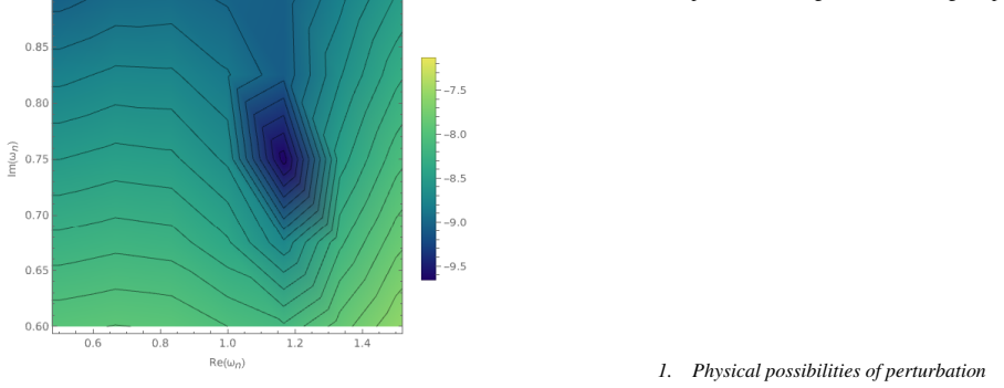
Physical possibilities of perturbation In the simplest cavity configurations, pseudospectrum anal- ysis indicates susceptibility to instability. However, this does not by itself clarify how the eigenvalues behave under physi- cally meaningful perturbations. To illustrate this point, Fig. 14 shows the spectrum of a cav- ity with the same parameters as in t...
2014
-
[7]
Permittivity of generic case following Lorentz model Making an educated assumption that the polarization is ex- ponentially dependent on time:P(t) =P 0e−iωt and inseting that in eq.5, we get the general form of a permittivity that fol- lows Lorentz model: (−ω2 −iΓω+w 2
-
[8]
for a recent contribution along these lines, extending the hyperboloidal scheme to the dispersive case with a focus on the study of dispersive extended theories of gravity). Second, we incorporate pseudospectrum analysis into the study of electromagnetic QNMs. While pseudospectra have been crucial to understand non-normal operators in jl fluid dy- namics ...
arXiv 2026
Show all 64 references
-
[9]
˜P=ω 2 pϵ∞E0 (A1) and then: ˜P E0 = ω2 pϵ∞ −ω2 −iΓω+w 2 0 (A2) On the other hand the relation between the electric field and the polarization is: P=ϵ 0χeE0,(A3) whereχ e is the electric susceptibility of the medium and it is related to its relative permittivity by the relation...
-
[10]
Having that makes a potential case a special ”mathe- matical” case of the permittivity one
Contact with a scattering by a potential PuttingΓto0(zero absorption) and plugging that in the QNMs wave equation we get: ∆E+ ϵ∞ c2 E−w 2 pE= 0(A6) Which is exactly the QNMs wave equation with a potential V=w 2 p. Having that makes a potential case a special ”mathe- matical” c...
1972
-
[11]
Chebyshev polynomials Chebyshev polynomials of the first kind are defined through the identity : Tk(cosθ) = cos(kθ)(B1) It can be written also for|x|<1as: Tk(x) = cos(k arccos(x))(B2) The following lines gives the few first Chebyshev polynomi- als: T0(x) = 1 T1(x) =x T2(x) = 2...
-
[12]
xj = cos( π(j+ 1 2 ) N+ 1 ) :j= 0,1,2, ...., N(B7) Andϕ j = π(j+ 1 2 ) N+1
Grids • Chebyshev-Gauss grid, where the points corresponds to the roots of Chebyshev polynomial. xj = cos( π(j+ 1 2 ) N+ 1 ) :j= 0,1,2, ...., N(B7) Andϕ j = π(j+ 1 2 ) N+1 . Note that this grid contains no boundary points,x 0 = cos( π 2N+2 )<1, andx N = −cos( π 2N+2 )>−1. • Ch...
-
[13]
(B24) 19
Chebyshev differential matrix Gauss D1 mj = xm 2(1−x2m) m=j (−1)m−j √ 1−x2 j (xm−xj ) √ 1−x2m m̸=j (B16) and those of the second order differentiation matrix: D2 mj = xm (1−x2m)2 − N(N+2) 3(1−x2m) m=j (−1)m−j √ 1−x2 j (xm−xj ) √ 1−x2m ( xm (1−x2m) − 2 xm−xj...
-
[14]
Chebyshev integration matrix To integrate a function over the space in a Lobatto grid, we can use the matrix Iij = cos πi Nz 2Nz + 1 + cos 2πi Nz 4Nz + NX k=2 2−δ k,N 2N cos πik Nz cos πi Nz +ksin πik Nz sin πi Nz...
-
[15]
Coordinate transformation Starting from the Bizo´n–Mach hyperboloidal coordinates τ=t−ln(2 coshx), y= tanh(x),(C1) the tangent vectors transform according to ∂t =∂ τ , ∂x =−y ∂τ + (1−y 2)∂ y. (C2)
-
[16]
Second-order derivatives From these relations, one computes ∂2 t =∂ 2 τ , ∂2 x =y 2 ∂2 τ −2y(1−y 2)∂ τ ∂y −(1−y 2)∂ τ −2y(1−y 2)∂ y + (1−y 2)∂ 2 y. (C3)
-
[17]
(18) of the main text
Differential operatorsL 1 andL 2 Inserting these expressions into the Maxwell–Lorentz sys- tem yields the operators L1 =−2y(1−y 2)∂y + (1−y 2)2∂2 y, L2 =−2y(1−y 2)∂y −(1−y 2)I, (C4) as given in Eq. (18) of the main text
-
[18]
This simplification transforms Maxwell’s curl equa- tions into one-dimensional derivatives while retaining the dis- persive structure
Scalar reduction In the one-dimensional reduction with fields aligned along a fixed axis, the vector fieldsEandPreduce to scalar fields EandP. This simplification transforms Maxwell’s curl equa- tions into one-dimensional derivatives while retaining the dis- persive structure....
-
[19]
Jaramillo, J.L., Panosso Macedo, R., Al Sheikh, L.: Pseu- dospectrum and black hole quasi-normal mode (in)stability (2020)
2020
-
[20]
Theses, Universit ´e Bourgogne Franche- Comt´e (2022)
Al Sheikh, L.: Scattering resonances and Pseudospectrum : stability and completeness aspects in optical and gravi- tational systems. Theses, Universit ´e Bourgogne Franche- Comt´e (2022). URLhttps://theses.hal.science/ tel-04116011
2022
-
[21]
Physical Review Letters110(23), 237,401 (2013)
Sauvan, C., Hugonin, J.P., Maksymov, I., Lalanne, P.: Theory of the spontaneous optical emission of nanosize photonic and plasmon resonators. Physical Review Letters110(23), 237,401 (2013)
2013
-
[22]
Muljarov, E.A., Weiss, T.: Resonant-state expansion for open optical systems: generalization to magnetic, chiral, and bi- anisotropic materials. Opt. Lett.43(9), 1978–1981 (2018). doi:10.1364/OL.43.001978. URLhttps://opg.optica. org/ol/abstract.cfm?URI=ol-43-9-1978
1978 doi
-
[23]
Laser & Photonics Reviews12(5), 1700,113 (2018)
Lalanne, P., Yan, W., Vynck, K., Sauvan, C., Hugo- nin, J.: Light interaction with photonic and plas- monic resonances. Laser & Photonics Reviews12(5), 1700,113 (2018). doi:10.1002/lpor.201700113. URL https://onlinelibrary.wiley.com/doi/abs/ 10.1002/lpor.201700113
2018 doi
-
[24]
SIAM Journal on Scientific Computing48(3), A1075–A1100 (2026)
Zengino ˘glu, A.: A null infinity layer for wave scattering. SIAM Journal on Scientific Computing48(3), A1075–A1100 (2026)
2026
-
[25]
arXiv preprint arXiv:2606.25130 (2026)
Wess, M., Zengino ˘glu, A.: Finite elements for helmholtz scat- tering with infinity as a computational boundary. arXiv preprint arXiv:2606.25130 (2026)
2026 arXiv
-
[26]
Frontiers in Physics Volume 12 - 2024(2024)
Burgess, C., K ¨onig, F.: Hyperboloidal method for quasinormal modes of non-relativistic operators. Frontiers in Physics Volume 12 - 2024(2024). doi:10.3389/fphy.2024.1457543. URLhttps://www.frontiersin.org/journals/ physics/articles/10.3389/fphy.2024.1457543
2024
-
[27]
Science261(5121), 578–584 (1993)
Trefethen, L.N., Trefethen, A.E., Reddy, S.C., Driscoll, T.A.: Hydrodynamic stability without eigenval- ues. Science261(5121), 578–584 (1993). doi: 10.1126/science.261.5121.578. URLhttps://science. sciencemag.org/content/261/5121/578
1993 doi
-
[28]
Princeton Uni- versity Press (2005)
Trefethen, L., Embree, M.: Spectra and Pseudospectra: The Be- havior of Nonnormal Matrices and Operators. Princeton Uni- versity Press (2005). URLhttps://books.google.es/ books?id=7gIbT-Y7-AIC
2005
-
[29]
Journal of Mathematical Physics56(10) (2015)
Krej ˇciˇr´ık, D., Siegl, P., Tater, M., Viola, J.: Pseudospectra in non-hermitian quantum mechanics. Journal of Mathematical Physics56(10) (2015). doi:10.1063/1.4934378
2015 doi
-
[30]
Colbrook, M.J., Roman, B., Hansen, A.C.: How to com- pute spectra with error control. Phys. Rev. Lett.122, 250,201 (2019). doi:10.1103/PhysRevLett.122.250201. URLhttps://link.aps.org/doi/10.1103/ PhysRevLett.122.250201
2019 doi
-
[31]
Frontiers in PhysicsVol- ume 13 - 2025(2026)
Bizo ´n, P., Gasper ´ın, E., Jaramillo, J.L.: Editorial: Quasi- normal modes, non-selfadjoint operators and pseudospectrum: an interdisciplinary approach. Frontiers in PhysicsVol- ume 13 - 2025(2026). doi:10.3389/fphy.2025.1753507. URLhttps://www.frontiersin.org/journals/ phys...
2025
-
[32]
Communications in Mathematical Physics306(1), 119–163 (2011)
Dyatlov, S.: Quasi-normal modes and exponential energy decay for the kerr-de sitter black hole. Communications in Mathematical Physics306(1), 119–163 (2011). doi: 10.1007/s00220-011-1286-x. URLhttps://doi.org/ 10.1007%2Fs00220-011-1286-x
2011 doi
-
[33]
Graduate Studies in Mathematics
Dyatlov, S., Zworski, M.: Mathematical Theory of Scatter- ing Resonances. Graduate Studies in Mathematics. Ameri- can Mathematical Society (2019). URLhttps://books. google.fr/books?id=atCuDwAAQBAJ
2019
-
[34]
Warnick, C.M.: On quasinormal modes of asymptotically anti- de Sitter black holes. Commun. Math. Phys.333(2), 959–1035 (2015). doi:10.1007/s00220-014-2171-1
2015 doi
-
[36]
Laser & Photonics Reviews19(9), 2402,133 (2025)
Wu, T., Jaramillo, J.L., Lalanne, P.: Reflections on the spa- tial exponential growth of electromagnetic quasinormal modes. Laser & Photonics Reviews19(9), 2402,133 (2025)
2025
-
[37]
Physical Review D98(12) (2018)
Macedo, R.P., Jaramillo, J.L., Ansorg, M.: Hyperboloidal slic- ing approach to quasinormal mode expansions: The reissner- nordstr¨om case. Physical Review D98(12) (2018). doi: 10.1103/physrevd.98.124005. URLhttp://dx.doi.org/ 10.1103/PhysRevD.98.124005
2018 doi
-
[38]
Classical and Quantum Gravity37(6), 065,019 (2020)
Macedo, R.P.: Hyperboloidal framework for the kerr spacetime. Classical and Quantum Gravity37(6), 065,019 (2020). doi: 10.1088/1361-6382/ab6e3e. URLhttps://dx.doi.org/ 10.1088/1361-6382/ab6e3e
2020 doi
-
[39]
Physical Review D83(12) (2011)
Zengino ˘glu, A.: A geometric framework for black hole perturbations. Physical Review D83(12) (2011). doi: 10.1103/physrevd.83.127502. URLhttp://dx.doi.org/ 10.1103/PhysRevD.83.127502
2011 doi
-
[40]
Bizo ´n, P., Mach, P.: Global dynamics of a Yang-Mills field on an asymptotically hyperbolic space. Trans. Am. Math. Soc.369(3), 2029–2048 (2017). doi: 10.1090/tran/6807, 10.1090/tran/7142. [Erratum: Trans. Am. Math. Soc.369,no.4,3013(2017)]
-
[41]
Donninger, R., Glogi ´c, I.: Strichartz estimates for the one- dimensional wave equation. Trans. Am. Math. Soc.373(6), 4051–4083 (2020). doi:10.1090/tran/8075
2020 doi
-
[42]
187 (2013)
Ansorg, M.: Spektrale verfahren in der theoretischen physik p. 187 (2013)
2013
-
[43]
Scientific Com- putation
Canuto, C., Hussaini, M., Quarteroni, A., Zang, T.: Spectral Methods: Fundamentals in Single Domains. Scientific Com- putation. Springer Berlin Heidelberg (2007). URLhttps: //books.google.es/books?id=DFJB0kiq0CQC
2007
-
[44]
Software, Envi- ronments, and Tools
Trefethen, L.: Spectral Methods in MATLAB. Software, Envi- ronments, and Tools. Society for Industrial and Applied Math- ematics (SIAM, 3600 Market Street, Floor 6, Philadelphia, PA 19104) (2000). URLhttps://books.google.es/ books?id=9Zu4YqPQKocC
2000
-
[45]
Progress of Theoretical Physics33(6), 1116–1128 (1965)
Hokkyo, N.: A remark on the norm of the unstable state: A role of adjoint wave functions in non-self-adjoint quantum systems. Progress of Theoretical Physics33(6), 1116–1128 (1965). doi:10.1143/PTP.33.1116. URLhttps://doi. org/10.1143/PTP.33.1116
1965 doi
-
[46]
American Journal of Physics42(4), 310–315 (1974)
Ohanian, H.C., Ginsburg, C.G.: Antibound ‘states’ and reso- nances. American Journal of Physics42(4), 310–315 (1974)
1974
-
[47]
Canadian Journal of Physics89(11), 1127–1140 (2011)
Belchev, B., Neale, S., Walton, M.: Flow of s-matrix poles for elementary quantum potentials1this research was supported in 21 part by an nserc undergraduate summer research award (sgn) and an nserc discovery grant (maw). Canadian Journal of Physics89(11), 1127–1140 (2011). do...
2011 doi
-
[48]
Siegert, A.J.F.: On the derivation of the dispersion for- mula for nuclear reactions. Phys. Rev.56, 750–752 (1939). doi:10.1103/PhysRev.56.750. URLhttps://link.aps. org/doi/10.1103/PhysRev.56.750
1939 doi
-
[49]
Zeitschrift f¨ur Physik204(212) (1928)
Gamow, G.: Zur quantentheorie des atomkernes. Zeitschrift f¨ur Physik204(212) (1928). doi:10.1007/BF01343196. URL https://doi.org/10.1007/BF01343196
1928 doi
-
[50]
Proceedings of the Royal Society of London
Peierls, R.E.: Complex eigenvalues in scattering the- ory. Proceedings of the Royal Society of London. Se- ries A. Mathematical and Physical Sciences253(1272), 16–36 (1959). doi:10.1098/rspa.1959.0176. URL https://royalsocietypublishing.org/doi/ abs/10.1098/rspa.1959.0176
1959
-
[51]
Pseudo- Differential Operators
Sj ¨ostrand, J.: Non-Self-Adjoint Differential Operators, Spec- tral Asymptotics and Random Perturbations. Pseudo- Differential Operators. Springer International Publishing (2019). URLhttps://books.google.es/books?id= 8QeZDwAAQBAJ
2019
-
[52]
Jaramillo, J.L., Macedo, R.P., Sheikh, L.A.: Gravita- tional wave signatures of black hole quasinormal mode in- stability. Phys. Rev. Lett.128, 211,102 (2022). doi: 10.1103/PhysRevLett.128.211102. URLhttps://link. aps.org/doi/10.1103/PhysRevLett.128.211102
2022 doi
-
[53]
doi:10.1088/1361-6382/ac5054
Gasper ´ın, E., Jaramillo, J.L.: Energy scales and black hole pseudospectra: the structural role of the scalar product 39(11), 115,010 (2022). doi:10.1088/1361-6382/ac5054. URLhttps://dx.doi.org/10.1088/1361-6382/ ac5054
2022 doi
-
[54]
General Relativity and Gravitation57(2025)
Besson, J., Jaramillo, J.L.: Quasi-normal mode expansions of black hole perturbations: a hyperboloidal keldysh’s ap- proach. General Relativity and Gravitation57(2025). doi: 10.1007/s10714-025-03438-6. URLhttps://doi.org/ 10.1007/s10714-025-03438-6
2025 doi
-
[55]
Bulletin of Mathemat- ical Sciences6(3), 379–452 (2016)
Ivrii, V .: 100 years of weyl’s law. Bulletin of Mathemat- ical Sciences6(3), 379–452 (2016). doi:10.1007/s13373- 016-0089-y. URLhttp://dx.doi.org/10.1007/ s13373-016-0089-y
2016 doi
-
[56]
Jaramillo, J.L., Macedo, R.P., Meneses-Rojas, O., Raf- faelli, B., Al Sheikh, L.: A weyl law for black holes. Phys. Rev. D110, 104,008 (2024). doi: 10.1103/PhysRevD.110.104008. URLhttps://link. aps.org/doi/10.1103/PhysRevD.110.104008
2024 doi
-
[57]
Frontiers in PhysicsVol- ume 12 - 2024(2025)
Panosso Macedo, R., Zengino ˘glu, A.: Hyperboloidal ap- proach to quasinormal modes. Frontiers in PhysicsVol- ume 12 - 2024(2025). doi:10.3389/fphy.2024.1497601. URLhttps://www.frontiersin.org/journals/ physics/articles/10.3389/fphy.2024.1497601
2024
-
[58]
Ansorg, M., Panosso Macedo, R.: Spectral decomposition of black-hole perturbations on hyperboloidal slices. Phys. Rev. D93(12), 124,016 (2016). doi:10.1103/PhysRevD.93.124016
2016 doi
-
[59]
Tellus24(3), 199–215 (1972)
Kreiss, H.O., Oliger, J.: Comparison of accurate methods for the integration of hyperbolic equations. Tellus24(3), 199–215 (1972)
1972
-
[60]
Studies in Applied Mathematics51(3), 253–259 (1972)
Orszag, S.A.: Comparison of pseudospectral and spectral ap- proximation. Studies in Applied Mathematics51(3), 253–259 (1972)
1972
-
[61]
The Physics of Fluids12(12), II–250 (1969)
Orszag, S.A.: Numerical methods for the simulation of turbu- lence. The Physics of Fluids12(12), II–250 (1969)
1969
-
[62]
SIAM Journal on Numerical Analysis21(4), 695– 715 (1984)
Dyksen, W.R., Houstis, E.N., Lynch, R.E., Rice, J.R.: The per- formance of the collocation and galerkin methods with hermite bi-cubics. SIAM Journal on Numerical Analysis21(4), 695– 715 (1984). URLhttp://www.jstor.org/stable/ 2157003
1984
-
[63]
Journal of Computational Physics27(3), 323–350 (1978)
Houstis, E.N., Lynch, R.E., Rice, J., Papatheodorou, T.: Evalu- ation of numerical methods for elliptic partial differential equa- tions. Journal of Computational Physics27(3), 323–350 (1978)
1978
-
[64]
Hussaini, M.Y ., Streett, C.L., Zang, T.A.: Spectral methods for partial differential equations (1983)
1983
-
[65]
Engineering Analysis with Boundary Elements27(3), 251–257 (2003)
Li, J., Cheng, A.H.D., Chen, C.S.: A comparison of efficiency and error convergence of multiquadric collocation method and finite element method. Engineering Analysis with Boundary Elements27(3), 251–257 (2003)
2003
Reviewed July 31, 2026 · model on record in the stance chip above.
Discussion (0). Continue with ORCID to comment.