REVIEW 3 major objections 5 minor 53 references
High-Resolution Dayside Spectroscopy of the Ultra-Hot Jupiter WASP-178b with GHOST/Gemini South
T0 review · 3 major / 5 minor · reviewed 2026-08-01 · deepseek-v4-flash
Pith's one-line read The paper reports an 8.3-sigma detection of neutral iron emission from the dayside of ultra-hot Jupiter WASP-178b, evidence of a thermal inversion in its atmosphere.
desk verdict The Fe emission detection is likely real and worth taking seriously, but the abstract's claim to 'verify a thermal inversion' overreaches because the template already assumes an inverted T-P profile. read the letter →
The pith
A machine-rendered reading of the paper's core claim, the machinery that carries it, and where it could break.
The reading
What carries the argument
The analysis hinges on Doppler cross-correlation against an LTE emission template built with a one-dimensional radiative-transfer model and an assumed solar-abundance chemical equilibrium composition. The template uses a two-point temperature-pressure profile taken from a prior retrieval of the same planet's near-infrared dayside spectrum; that profile itself contains the thermal inversion the paper argues the emission verifies. The cross-correlation map in Keplerian-velocity versus radial-velocity space is the mechanism that separates a genuine planetary signal from telluric and stellar contamination, and the model injection/recovery tests quantify how well the template matches the data.
What would settle it
Cross-correlate the same data with a template computed from a self-consistent non-LTE temperature-pressure profile (for example, one that produces a cooler upper atmosphere). If the 8.3σ peak disappears or flips to absorption, the inversion claim fails; if it persists, the inversion is robust.
Extended reading notes
Core claim
The central claim is a strong (8.3σ) detection of neutral atomic iron in emission from the dayside of WASP-178b, found by Doppler cross-correlating high-resolution optical spectra with a model generated under local thermodynamic equilibrium (LTE). The correlation peak sits at a Keplerian velocity of 175.0(+2.3/−2.6) km/s and near-zero radial velocity, matching the expected planetary motion. Because an inverted temperature-pressure profile is required for iron to appear in emission rather than absorption, the authors interpret the detection as verification of a thermal inversion in the dayside atmosphere, complementing a previous near-infrared study. They also report tentative (≈4σ) hints of
Load-bearing premise
The interpretation that the signal is iron emission from a thermal inversion depends on the adopted two-point temperature-pressure profile (already containing the inversion) and the LTE template; if the template misrepresents line formation, the signal's sign or significance could change.
Editorial extensions
If this is right
- If the detection is correct, neutral iron survives on the dayside despite temperatures high enough to ionize it, constraining the ionization balance and vertical mixing.
- The emission signature confirms a thermal inversion in the optical, extending the evidence previously available only from near-infrared CO and H2O detections.
- The tentative silicon emission adds a new data point to the small set of ultra-hot Jupiters with dayside Si detections, supporting the idea that SiO from cooler regions dissociates on the hottest dayside.
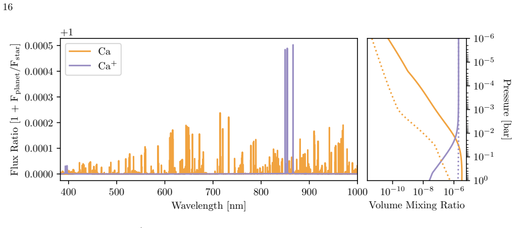
- The tentative calcium emission, with no corresponding Ca+ detection, suggests the observations probe pressures near the Ca/Ca+ ionization boundary.
- Joint analysis with existing near-infrared dayside spectra could yield a refractory-to-volatile abundance ratio, linking composition to planet formation.
Reading between the lines
- A natural next step is a non-LTE emission template; if the inversion is as strong as recent non-LTE simulations suggest, the iron lines might be even brighter than LTE predicts, and the injection/recovery discrepancy (5.1σ recovered vs 7.7σ observed) hints the LTE template under-predicts the signal.
- If the silicon hint is real and confined to pre-eclipse phases, it would imply Si is concentrated near the dayside hotspot, tracing the dissociation of SiO into a gaseous Si reservoir that could later condense into silicate clouds on the nightside.
- The slight offset in the calcium peak's Keplerian velocity (167 vs 176 km/s) could indicate that different species probe different atmospheric layers with different wind dynamics; a longer phase coverage would test this.
Editorial analysis
A structured set of objections, weighed in public.
Referee Report
Summary. This paper presents ~9 h of GHOST/Gemini South high-resolution optical spectroscopy of the ultra-hot Jupiter WASP-178b, obtained at pre- and post-eclipse phases (272 exposures). After DRAGONS reduction and SysRem telluric/stellar removal, the authors perform Doppler cross-correlation of the data with 1D LTE petitRADTRANS/FastChem models built from a two-point T-P profile taken from the CRIRES+ retrieval of Cont et al. (2024). They report an 8.3σ detection of Fe at Kp = 175.0^{+2.3}_{-2.6} km/s and RV = -0.9^{+1.8}_{-1.3} km/s, tentative 4.0σ Si and 4.3σ Ca signals, and non-detections for the other 11 species searched. Injection/recovery tests show that only Fe (and marginally Ca in one arm) can be recovered at the expected location. The authors interpret the Fe emission as verifying a dayside thermal inversion in WASP-178b.
Significance. The Fe detection, if taken at face value, is a valuable addition to high-resolution dayside spectroscopy of ultra-hot Jupiters: it is the first high-resolution optical dayside Fe detection for WASP-178b, and the measured Kp is consistent with previous transmission-spectroscopy measurements, strengthening the case for a planetary origin. The paper is also transparent in several respects: the ΔCCF-based SysRem iteration optimization is described in detail, the injection/recovery results are reported honestly even when they show model mismatch, and the reduced data are made available in the Gemini archive. However, the central interpretive claim that this detection 'verifies' a thermal inversion is not supported by the analysis as presented, because the Fe template already assumes an inverted T-P profile. The detection is better characterized as consistent with the assumed inverted template or with a thermal inversion; the paper needs either a control calculation or a change in wording to avoid circularity.
major comments (3)
- [§4, Table 1, §7.1] The Fe emission template is constructed with petitRADTRANS using the two-point T-P profile from Cont et al. (2024): T1 = 3661 K at log p1 = −4.62 and T2 = 2756 K at log p2 = −0.33 (Table 1). This profile already contains a thermal inversion. The abstract and §7.1 claim that the 8.3σ detection 'verifies' that inversion. That inference is circular unless a control model without an inversion is also cross-correlated, because a positive CCF peak for the inverted-profile template is exactly what the assumed profile predicts. I request either (a) an additional cross-correlation with a non-inverted (e.g., isothermal or monotonically decreasing) Fe template, reporting the CCF sign and significance, or (b) revision of the abstract/conclusions to state that the detection is consistent with, but does not independently verify, a thermal inversion.
- [§5.1, §6.1] The detection significance is computed as the peak divided by the standard deviation of a 3σ-clipped version of the same Kp−RV map. This does not account for the large search space (Kp from 1 to 300 km/s in 1 km/s steps, RV from −300 to +300 km/s) or for the fact that 14 species were tested. The quoted 8.3σ should be accompanied by a null-hypothesis calibration (e.g., bootstrap or velocity-scrambled noise maps) or a formal look-elsewhere correction. The tentative 4.0σ Si and 4.3σ Ca peaks in the same maps are especially sensitive to this issue; without such calibration the meaning of the 5σ 'confident detection' threshold is not well defined.
- [§6.3] The injection/recovery test recovers an injected Fe model at only 5.1σ in the night-1 red data, compared with the observed 7.7σ in the same arm. As the authors note, this indicates the 1D LTE template is not a good match to the true line shape. Consequently, the quoted 8.3σ and the emission/inversion interpretation are template-dependent. The paper does not test whether the observed features would also be consistent with a non-inverted LTE template or with NLTE line formation. I recommend either adding a sign/amplitude fit for Fe (e.g., fitting the CCF with a free continuum and emission/absorption scaling) or explicitly quantifying how much of the 8.3σ relies on the inverted-profile assumption.
minor comments (5)
- [Abstract and title] The manuscript consistently renders 'WASP-178b' as 'W ASP-178b' in the title, abstract, and body text. Please correct the spacing throughout.
- [§2] The text states that sky subtraction and barycentric correction were turned OFF, then says BERV values were taken from the default products. Please clarify whether the default DRAGONS products were used only for BERV and not for the spectra used in the analysis.
- [Figure 5 caption] The caption says 'dashed black lines represent the combined peak RV and Kp' but the plotted slices are not individually labeled with units. Adding numerical peak values and units would improve readability.
- [§4] Please state explicitly in §4 that all models are 1D, LTE, solar-abundance, and that no limb/dayside viewing-angle weighting is applied. This is acknowledged later in §7.3, but it should be stated where the models are introduced.
- [References] Some inline citations use inconsistent formats, e.g., 'Talens, G. J. J. et al.' rather than the author-year format used elsewhere. A thorough copyedit is needed.
Circularity Check
Fe detection likely real, but 'verify thermal inversion' is self-referential because the emission template already encodes the inverted T-P profile.
-
self definitional
[Abstract; Section 4; Section 7.1]
"We verify the presence of a thermal inversion in the dayside atmosphere with a high-significance (8.3σ) detection of neutral iron emission ... the T-P profile was generated using the best-fit parameters from the retrieval analysis of a two-point T-P profile presented in D. Cont et al. (2024). ... The fact that we observe Fe in emission is also consistent with the presence of a thermal inversion in WASP-178b’s atmosphere, as first demonstrated by D. Cont et al. (2024)."
The Fe emission template used for cross-correlation is constructed from a two-point T-P profile (T1=3661 K at log p1=-4.62, T2=2756 K at log p2=-0.33) that already contains the thermal inversion. This fixes the sign of the model lines as emission; a positive CCF then merely indicates the data contain the template's line pattern, not that the inversion is independently detected. Without a control using a non-inverted (absorption) template, the claim to 'verify' the inversion reduces to the assumption already built into the model.
full rationale
The paper's detection of Fe at 8.3σ is a genuine cross-correlation signal at the expected Kp, and the injection/recovery test shows the observed signal is stronger than the injected model (7.7σ vs 5.1σ), so the detection is not merely the model fitting itself. However, the interpretation of this signal as iron emission, and hence as verification of a thermal inversion, is contingent on the inverted T-P profile adopted from Cont et al. (2024) to generate the template. Because the template's emission/absorption contrast is determined by that assumed profile, the positive correlation does not independently prove the inversion; it is self-referential. The paper also acknowledges the inversion was 'first demonstrated' by Cont et al., so the verification is partially redundant. No fitted parameters are derived from the detection, and the species detection itself is likely robust, so the circularity is moderate rather than severe.
Assumptions & free parameters
free parameters (2)
- Two-point T-P profile anchors (T1, log p1; T2, log p2) =
T1=3661 K, log p1=-4.62 (+1.56/-1.88); T2=2756 K, log p2=-0.33 (+1.64/-1.53)
- SysRem iteration counts (per camera/night) =
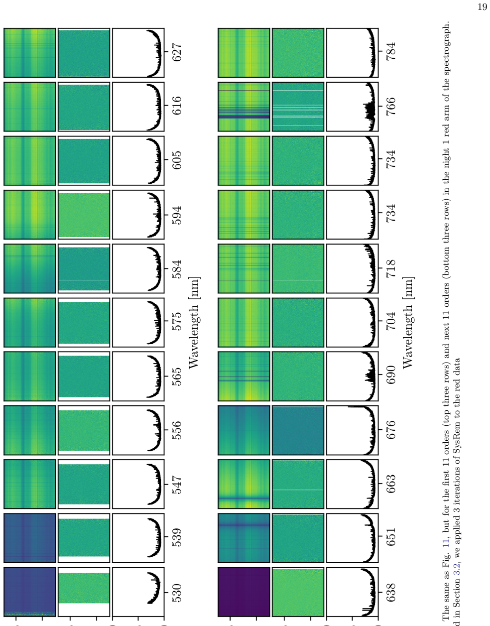
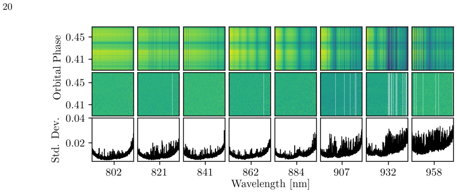
red N1=2, red N2=3; blue N1=N2=5
assumptions (5)
- domain assumption LTE, 1D, solar-abundance chemical-equilibrium emission models with adopted line lists are adequate CCF templates.
- domain assumption SysRem removes time-stationary stellar/telluric features without removing the planetary signal.
- domain assumption The sigma-clipped standard deviation of the 2D Kp-RV map is a valid noise estimate for computing CCF significances.
- domain assumption The adopted line lists (Fe, Si, Ca, Ca+, etc.) are accurate over the GHOST usable wavelength range.
- domain assumption The planet's emitting region follows the adopted Keplerian velocity with no strong wind-induced distortion.
Cite this review
Pith. "Pith review of High-Resolution Dayside Spectroscopy of the Ultra-Hot Jupiter WASP-178b with GHOST/Gemini South." pith.science (2026). https://pith.science/paper/O4P6WZUN
@misc{pith2026260727363,
  author       = {Pith},
  title        = {Pith review of: High-Resolution Dayside Spectroscopy of the Ultra-Hot Jupiter WASP-178b with GHOST/Gemini South},
  year         = {2026},
  howpublished = {\url{https://pith.science/paper/O4P6WZUN}},
  note         = {Machine review of arXiv:2607.27363}
}
abstract
We present high-resolution dayside spectroscopy of the ultra-hot Jupiter WASP-178b obtained with the Gemini High-resolution Optical SpecTrograph (GHOST) at the Gemini South Observatory. The observations cover pre- and post-eclipse orbital phases, lasting approximately 9 hours in total, and represent the first published high-resolution optical dayside emission spectroscopy of WASP-178b's atmosphere, complementing previous near-infrared dayside spectroscopy. We verify the presence of a thermal inversion in the dayside atmosphere with a high-significance (8.3$\sigma$) detection of neutral iron emission via the Doppler cross-correlation technique, alongside hints of neutral Si and Ca emission. We also carry out model injection/recovery tests for other atmospheric species, which indicate that we do not expect to detect the majority of species searched for in this work, assuming our models are accurate representations of the planet's atmosphere. Finally, we place our results into context with previous work, showing how our tentative detection of neutral Si complements existing space-based observations and adds a new data point to previous detections of Si in ultra-hot Jupiter atmospheres. Our high-resolution observations provide important context about the dayside of WASP-178b, shedding light on 3D atmospheric processes and the extreme conditions present in ultra-hot Jupiter atmospheres.
Figures


Figures from the paper (13 more)





Reference graph
Works this paper leans on
-
[1]
Astropy Collaboration, Robitaille, T. P., Tollerud, E. J., et al. 2013, A&A, 558, A33, doi: 10.1051/0004-6361/201322068 Astropy Collaboration, Price-Whelan, A. M., Sip˝ ocz, B. M., et al. 2018, AJ, 156, 123, doi: 10.3847/1538-3881/aabc4f Astropy Collaboration, Price-Whelan, A. M., Lim, P. L., et al. 2022, ApJ, 935, 167, doi: 10.3847/1538-4357/ac7c74
-
[2]
Bell, T. J., & Cowan, N. B. 2018, The Astrophysical Journal Letters, 857, L20, doi: 10.3847/2041-8213/aabcc8
-
[3]
Buchhave, L. A., & Rathcke, A. D. 2022, AJ, 163, 96, doi: 10.3847/1538-3881/ac402e
-
[4]
Bonidie, V., Johnson, M. C., Wang, J., et al. 2026, AJ, 171, 34, doi: 10.3847/1538-3881/ae21be
-
[5]
2021, A&A, 645, A24, doi: 10.1051/0004-6361/202039344
Borsa, F., Allart, R., Casasayas-Barris, N., et al. 2021, A&A, 645, A24, doi: 10.1051/0004-6361/202039344
-
[6]
Brogi, M., & Line, M. R. 2019, AJ, 157, 114, doi: 10.3847/1538-3881/aaffd3
-
[7]
2019, A&A, 628, A9, doi: 10.1051/0004-6361/201935623
Casasayas-Barris, N., Pall´ e, E., Yan, F., et al. 2019, A&A, 628, A9, doi: 10.1051/0004-6361/201935623
-
[8]
A., Lothringer, J., & Blake, G
Chachan, Y., Knutson, H. A., Lothringer, J., & Blake, G. A. 2023, ApJ, 943, 112, doi: 10.3847/1538-4357/aca614
Show all 53 references
-
[9]
J., Madhusudhan, N., & Holmberg, M
Cheverall, C. J., Madhusudhan, N., & Holmberg, M. 2023, MNRAS, 522, 661, doi: 10.1093/mnras/stad648 18 Figure 11.The results of applying the SysRem algorithm to the first 11 orders (top three rows) and last 10 orders (bottom three rows) in the night 1 blue arm of the spectrogr...
2023 doi
-
[10]
2022, A&A, 657, L2, doi: 10.1051/0004-6361/202142776
Cont, D., Yan, F., Reiners, A., et al. 2022, A&A, 657, L2, doi: 10.1051/0004-6361/202142776
2022 doi
-
[11]
2024, https://arxiv.org/abs/2406.08166
Cont, D., Nortmann, L., Yan, F., et al. 2024, https://arxiv.org/abs/2406.08166
2024 arXiv
-
[12]
C., Seidel, J
Damasceno, Y. C., Seidel, J. V., Prinoth, B., et al. 2024, doi: https://doi.org/10.1051/0004-6361/202450119 D’Arpa, M. C., Saba, A., Borsa, F., et al. 2024, A&A, 690, A237, doi: 10.1051/0004-6361/202449341
2024 doi
-
[13]
K., Langeveld, A
Deibert, E. K., Langeveld, A. B., Young, M. E., et al. 2024, AJ, 168, 148, doi: 10.3847/1538-3881/ad643f
2024 doi
-
[14]
2017, AJ, 153, 268, doi: 10.3847/1538-3881/aa7133
Watson, C., & de Kok, R. 2017, AJ, 153, 268, doi: 10.3847/1538-3881/aa7133
2017 doi
-
[15]
J., Dawson, R
Fortney, J. J., Dawson, R. I., & Komacek, T. D. 2021, Journal of Geophysical Research: Planets, 126, e2020JE006629, doi: https://doi.org/10.1029/2020JE006629
2021 doi
-
[16]
E., Shulyak, D., et al
Fossati, L., Young, M. E., Shulyak, D., et al. 2021, A&A, 653, A52, doi: 10.1051/0004-6361/202140813
2021 doi
-
[17]
G., et al
Fossati, L., Shulyak, D., Sreejith, A. G., et al. 2020, A&A, 643, A131, doi: 10.1051/0004-6361/202039061
2020 doi
-
[18]
G., Koskinen, T., et al
Fossati, L., Sreejith, A. G., Koskinen, T., et al. 2025, A&A, 699, A186, doi: 10.1051/0004-6361/202554240
2025 doi
-
[19]
S., Stassun, K
Gaudi, B. S., Stassun, K. G., Collins, K. A., et al. 2017, Nature, 546, 514–518, doi: 10.1038/nature22392
2017 doi
-
[20]
2026, A&A, 706, A126, doi: 10.1051/0004-6361/202557869
Guo, B., Yan, F., Henning, T., et al. 2026, A&A, 706, A126, doi: 10.1051/0004-6361/202557869
2026 doi
-
[21]
R., Millman, K
Harris, C. R., Millman, K. J., van der Walt, S. J., et al. 2020, Nature, 585, 357, doi: 10.1038/s41586-020-2649-2
2020 doi
-
[22]
R., Barkaoui, K., et al
Hellier, C., Anderson, D. R., Barkaoui, K., et al. 2019, Monthly Notices of the Royal Astronomical Society, 490, 1479–1487, doi: 10.1093/mnras/stz2713
2019 doi
-
[23]
2019, A&A, 626, A133, doi: 10.1051/0004-6361/201834085
Helling, C., Gourbin, P., Woitke, P., & Parmentier, V. 2019, A&A, 626, A133, doi: 10.1051/0004-6361/201834085
2019 doi
-
[24]
P., & Jayawardhana, R
Gibson, N. P., & Jayawardhana, R. 2022, AJ, 163, 248, doi: 10.3847/1538-3881/ac5f4d
2022 doi
-
[25]
J., Kitzmann, D., Morris, B
Hoeijmakers, H. J., Kitzmann, D., Morris, B. M., et al. 2024, A&A, 685, A139, doi: 10.1051/0004-6361/202244968
2024 doi
-
[26]
Hunter, J. D. 2007, Computing in Science & Engineering, 9, 90, doi: 10.1109/MCSE.2007.55
2007 doi
-
[27]
M., Diaz, R
Kalari, V. M., Diaz, R. J., Robertson, G., et al. 2024, AJ, 168, 208, doi: 10.3847/1538-3881/ad72ed
2024 doi
- [28]
-
[29]
Turner, J. E. H. 2019, in Astronomical Society of the Pacific Conference Series, Vol. 523, Astronomical Data Analysis Software and Systems XXVII, ed. P. J. Teuben, M. W. Pound, B. A. Thomas, & E. M. Warner, 321
2019
-
[30]
2022,, 3.0.4, Zenodo Zenodo, doi: 10.5281/zenodo.7308726
Labrie, K., Simpson, C., Anderson, K., et al. 2022,, 3.0.4, Zenodo Zenodo, doi: 10.5281/zenodo.7308726
2022 doi
-
[31]
B., Deibert, E
Langeveld, A. B., Deibert, E. K., Young, M. E., et al. 2025, ApJL, 981, L32, doi: 10.3847/2041-8213/adb70d
2025 doi
-
[32]
D., Rustamkulov, Z., Sing, D
Lothringer, J. D., Rustamkulov, Z., Sing, D. K., et al. 2021, ApJ, 914, 12, doi: 10.3847/1538-4357/abf8a9
2021 doi
-
[33]
D., Sing, D
Lothringer, J. D., Sing, D. K., Rustamkulov, Z., et al. 2022, Nature, 604, 49, doi: 10.1038/s41586-022-04453-2
2022 doi
-
[34]
D., Bennett, K
Lothringer, J. D., Bennett, K. A., Sing, D. K., et al. 2025, The Astronomical Journal, 169, 274, doi: 10.3847/1538-3881/adc117
2025 doi
-
[35]
P., Nugroho, S
Maguire, C., Gibson, N. P., Nugroho, S. K., et al. 2023, MNRAS, 519, 1030, doi: 10.1093/mnras/stac3388 Mart ´ ınez, R. R., Gaudi, B. S., Rodriguez, J. E., et al. 2020, The Astronomical Journal, 160, 111, doi: 10.3847/1538-3881/ab9f2d 21 Figure 14.The same as Fig. 11, but for t...
2023 doi
-
[36]
W., Hayes, C
McConnachie, A. W., Hayes, C. R., Robertson, J. G., et al. 2024, PASP, 136, 035001, doi: 10.1088/1538-3873/ad1ed4 Molli` ere, P., Wardenier, J. P., van Boekel, R., et al. 2019, A&A, 627, A67, doi: 10.1051/0004-6361/201935470
2024 doi
-
[37]
K., Gibson, N
Nugroho, S. K., Gibson, N. P., de Mooij, E. J. W., et al. 2020, MNRAS, 496, 504, doi: 10.1093/mnras/staa1459
2020 doi
-
[38]
R., Bean, J
Parmentier, V., Line, M. R., Bean, J. L., et al. 2018, A&A, 617, A110, doi: 10.1051/0004-6361/201833059
2018 doi
-
[39]
2023, Nature, 619, 491, doi: 10.1038/s41586-023-06134-0
Pelletier, S., Benneke, B., Ali-Dib, M., et al. 2023, Nature, 619, 491, doi: 10.1038/s41586-023-06134-0
2023 doi
-
[40]
J., Pelletier, S., et al
Prinoth, B., Hoeijmakers, H. J., Pelletier, S., et al. 2023, A&A, 678, A182, doi: 10.1051/0004-6361/202347262
2023 doi
-
[41]
V., Hoeijmakers, H
Prinoth, B., Seidel, J. V., Hoeijmakers, H. J., et al. 2025, A&A, 694, A284, doi: 10.1051/0004-6361/202452405
2025 doi
-
[42]
2023, AJ, 165, 211, doi: 10.3847/1538-3881/acc654
Ridden-Harper, A., de Mooij, E., Jayawardhana, R., et al. 2023, AJ, 165, 211, doi: 10.3847/1538-3881/acc654
2023 doi
-
[43]
Saha, S., & Jenkins, J. S. 2025, arXiv e-prints, arXiv:2510.11479, doi: 10.48550/arXiv.2510.11479
2025 doi
-
[44]
A., Smith, P
Sanchez, J. A., Smith, P. C. B., Kanumalla, K., et al. 2025, arXiv e-prints, arXiv:2512.10904, doi: 10.48550/arXiv.2512.10904
2025 doi
-
[45]
Smith, P. C. B., Sanchez, J. A., Line, M. R., et al. 2024, AJ, 168, 293, doi: 10.3847/1538-3881/ad8574
2024 doi
-
[46]
2010, Nature, 465, 1049, doi: 10.1038/nature09111
Albrecht, S. 2010, Nature, 465, 1049, doi: 10.1038/nature09111
2010 doi
-
[47]
W., Kitzmann, D., Patzer, A
Stock, J. W., Kitzmann, D., Patzer, A. B. C., & Sedlmayr, E. 2018, MNRAS, 479, 865, doi: 10.1093/mnras/sty1531
2018 doi
-
[48]
Talens, G. J. J., Justesen, A. B., Albrecht, S., et al. 2018, A&A, 612, A57, doi: 10.1051/0004-6361/201731512
2018 doi
-
[49]
2005, MNRAS, 356, 1466, doi: 10.1111/j.1365-2966.2004.08585.x
Tamuz, O., Mazeh, T., & Zucker, S. 2005, MNRAS, 356, 1466, doi: 10.1111/j.1365-2966.2004.08585.x
2005
-
[50]
D., de Mooij, E
Turner, J. D., de Mooij, E. J. W., Jayawardhana, R., et al. 2020, ApJL, 888, L13, doi: 10.3847/2041-8213/ab60a9 van Sluijs, L., Rauscher, E., Kempton, E. M.-R., et al. 2025, AJ, 170, 217, doi: 10.3847/1538-3881/adfb61
2020 doi
-
[51]
E., et al
Virtanen, P., Gommers, R., Oliphant, T. E., et al. 2020, Nature Methods, 17, 261, doi: 10.1038/s41592-019-0686-2
2020 doi
-
[52]
2019, A&A, 632, A69, doi: 10.1051/0004-6361/201936396
Yan, F., Casasayas-Barris, N., Molaverdikhani, K., et al. 2019, A&A, 632, A69, doi: 10.1051/0004-6361/201936396
2019 doi
-
[53]
P., Householder, A., et al
Zhang, Y., Wardenier, J. P., Householder, A., et al. 2026, ApJL, 997, L40, doi: 10.3847/2041-8213/ae36a1
2026 doi
Reviewed August 1, 2026 · model on record in the stance chip above.
Discussion (0). Sign in to comment.