REVIEW 4 major objections 5 minor 38 references
Large-Time-Step Operation in a Volume Integral Equation for Dielectric Scattering
T0 review · 4 major / 5 minor · reviewed 2026-08-15 · deepseek-v4-flash
Pith's one-line read A marching-on-in-time volume integral solver for dielectric scattering takes time steps up to 16 times the CFL reference and shifts its dominant cost to an FFT-accelerated present-time matrix.
desk verdict Competent, useful incremental advance in large-time-step MOT-JVIE, but the 16× accuracy claim is under-supported by pointwise checks and a missing global error norm. read the letter →
The pith
A machine-rendered reading of the paper's core claim, the machinery that carries it, and where it could break.
The reading
What carries the argument
The load-bearing object is the present-time interaction matrix $\mathbf{Z}_0$ and its decomposition $\mathbf{Z}_0 = \mathbf{D} - \mathbf{X}\mathbf{G}$, where $\mathbf{D}$ and $\mathbf{X}$ are diagonal matrices for local constitutive and material-contrast terms and $\mathbf{G}$ is the volume-integral Green-function operator. Because the voxel grid is uniform and the background is homogeneous, the entries of $\mathbf{G}$ depend only on relative source--observer voxel offsets, giving it a multilevel block Toeplitz structure; embedding it in a circulant operator lets each matrix--vector product be computed by zero-padding, forward three-dimensional FFT, spectral multiplication with precomputed kernels, inverse FFT, and truncation back to the physical grid. This matrix-free application of $\mathbf{Z}_0$ is what removes the large-time-step bottleneck. The temporal admissibility condition $\Delta t \le 1/(2\kappa f_{\max})$ with $\kappa=2$ is what licenses the 16$\times$ step in the first place, together with quadratic-spline temporal basis functions and TFQMR iteration for the implicit marching system.
What would settle it
Run the 200 nm homogeneous cube with $\varepsilon_r=12$ at $\Delta t = 16\,\Delta t_{\mathrm{CFL}}$ and compute the global relative $\ell^2$ error between the $\alpha=16$ and $\alpha=1$ solutions over all voxels and all time steps; if that global error is large even though single-point traces agree, the claim that 16$\times$ steps are accurate for band-limited excitations is falsified.
Extended reading notes
Core claim
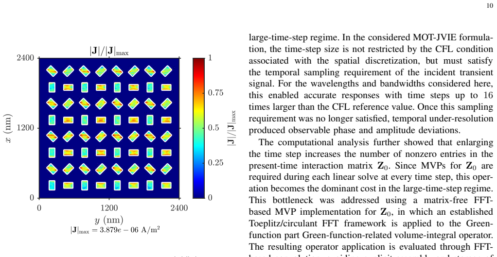
The central discovery is that in a marching-on-in-time current-density volume integral equation (MOT-JVIE) solver, the time step is limited by the Nyquist sampling of the band-limited incident and scattered fields rather than by a CFL stability condition, and that choosing $\Delta t = 16\,\Delta t_{\mathrm{CFL}}$ preserves accurate transient responses for the pulses considered. As the time step grows, the spherical causal wavefront that fills the present-time matrix in one step encloses more of the voxelized scatterer, so $\mathbf{Z}_0$ densifies rapidly. The paper shows the cost of the iterative linear solve then dominates, while TFQMR iteration counts stay low, pinpointing the matrix--vector product with $\mathbf{Z}_0$ as the true cost driver. That product is evaluated without forming $\mathbf{Z}_0$ by writing $\mathbf{Z}_0 = \mathbf{D} - \mathbf{X}\mathbf{G}$ and applying $\mathbf{G}$ as a multilevel Toeplitz/circulant convolution through three-dimensional FFTs, cutting the operator application to $\mathcal{O}(N\log N)$ and removing the memory ceiling of explicit sparse storage. Evidence includes matching current-density traces, normalized pointwise errors near $10^{-4}$, up to 15$\times$ speedups, and a full $8\times8$ GST/a-Si nanopillar array simulation with roughly $1.56\times10^{7}$ vector unknowns in single-threaded execution.
Load-bearing premise
The load-bearing premise is that the incident and scattered fields are effectively band-limited and that the oversampling factor $\kappa=2$ in the sampling condition is sufficient to guarantee the claimed transient accuracy; if that sampling assumption fails, the 16$\times$ time-step claim no longer applies.
Editorial extensions
If this is right
- Band-limited transient dielectric scattering can be marched with up to 16 times fewer time steps than the voxel-CFL reference, directly reducing time-marching, storage, and history-accumulation cost.
- In the large-time-step regime, further acceleration should target the present-time operator $\mathbf{Z}_0$ rather than history terms; the FFT-based Toeplitz/circulant application scales as $\mathcal{O}(N\log N)$ and never forms $\mathbf{Z}_0$ explicitly.
- The matrix-free present-time product lifts the memory wall that makes direct MOT-JVIE impractical for large metasurface arrays, demonstrated at about 15.6 million vector unknowns on a single CPU thread.
- Because TFQMR iteration counts remain low and stable as the time step grows, the FFT speedup is not eroded by slower convergence in the tested cases.
Reading between the lines
- The same bandwidth-limited large-time-step picture should carry over to other volume integral formulations on uniform grids — magnetic, dispersive, or nonlinear materials — whenever the Green-function operator retains Toeplitz structure; the paper's scalar nondispersive permittivity is a simplifying choice, not the mechanism.
- The accuracy ceiling is the Nyquist condition with $\kappa=2$: the paper's own $\alpha=32$ result shows the method is bandwidth-limited rather than unconditionally stable, so a user must know the effective $f_{\max}$ of the excitation before choosing $\Delta t$.
- FFT-based $\mathbf{Z}_0$ application should combine naturally with plane-wave time-domain or hierarchical FFT history acceleration, potentially also speeding up moderate-time-step regimes where neither history terms nor $\mathbf{Z}_0$ alone dominate.
- A global relative $\ell^2$ error over all voxels and all time steps, rather than pointwise traces, would settle how much conservatism is hidden in the $\kappa=2$ oversampling choice.
Signed reviews
Editorial analysis
A structured set of objections, weighed in public.
Referee Report
Summary. The manuscript studies large-time-step operation of a marching-on-in-time contrast-current-density volume integral equation (MOT-JVIE) for transient dielectric scattering. The time step is chosen by a Nyquist sampling condition (Eq. (5)) rather than by the CFL limit of the spatial voxel grid, and the paper demonstrates, for band-limited excitations, accurate solutions for time steps up to 16 times the reference CFL-limited step. A central computational observation is that as the time step grows, the present-time interaction matrix Z0 densifies, so the dominant cost shifts from history-term evaluations to repeated Z0 matrix-vector products inside the iterative solver. To address this, the authors apply a matrix-free FFT-based evaluation of Z0 exploiting its multilevel Toeplitz structure, and demonstrate more than an order-of-magnitude speedup on a cubic test case plus a single-threaded simulation of an 8x8 bilayer nanopillar metasurface with about 15.6 million unknowns.
Significance. If the accuracy and efficiency claims hold, the paper would be a substantial practical advance: it identifies a regime change in MOT-JVIE solvers, provides a concrete FFT-based remedy, and gives a credible large-scale demonstration without parallel hardware. The manuscript has notable strengths: the mathematical core (Toeplitz/circulant FFT MVP) is standard and the pointwise comparison against the direct sparse implementation at the 1e-4 level is a useful consistency check; there are no fitted parameters; and the use of an independent MOD-JVIE reference for the benchmark cube provides some external grounding. The main weakness is that the central accuracy claim is supported only by pointwise or single-observation-point comparisons, despite the paper explicitly promising a global relative l2-norm error in Section V-A.
major comments (4)
- [Section V-A and Fig. 10] The text at the start of Section V-A states that the comparison is performed 'in terms of induced contrast current density, relative ℓ2-norm error, runtime, and TFQMR convergence,' but no global relative ℓ2-norm error is ever reported. The only accuracy plot is Fig. 10(b), a normalized pointwise error at a single voxel and only for α=1. Since the direct implementation is available for the cube, please add the global relative ℓ2-norm error of the current-density vector over all voxels and all time steps for α=2, 4, 8, and 16, and indicate where in the domain and at which times the error is largest.
- [Section III-B and Fig. 3] The large-time-step accuracy claim is validated by one current-density component at voxel (41,41,41) for the homogeneous cube and by one azimuthal component at one observation point for the benchmark cube. These single-point checks do not by themselves support the abstract's global statement that 'accurate transient analysis is demonstrated for time steps up to 16 times larger.' Please provide a multi-voxel or global error assessment, ideally a convergence table in α for both the coarse and fine voxelizations, and explicitly check late-time behavior and regions near material discontinuities.
- [Section III-B, Eq. (5)] Equation (5) is a Nyquist criterion on the incident-field bandwidth; it does not by itself guarantee that the full MOT-JVIE solution is temporally accurate, because the temporal discretization also involves the quadratic-spline basis and the retarded Green-function interaction. The sufficiency of κ=2 should be demonstrated by a time-step convergence study, not inferred from the sampling formula alone. The observed degradation at α=32 in Fig. 3(b) is consistent with the Nyquist bound, but it does not quantify how close α=16 is to the accuracy threshold; a global error-versus-α curve would settle this.
- [Section V-B] The 8x8 nanopillar-array demonstration includes no quantitative accuracy check: Fig. 12 illustrates a spatial current pattern, but there is no comparison against a reference solution or a converged solution on a coarser or smaller problem. Because the array result is the flagship scalability claim, please add a validation step (for example, a smaller 2x2 or 4x4 array computed with the direct sparse implementation, or a coarse-grid comparison) to show that the FFT-based large-time-step solver retains the accuracy established for the cube.
minor comments (5)
- [Title/header] The title and running header contain a typo: 'V olume' should be 'Volume.'
- [Throughout] The manuscript uses 'MOT-JVIE,' 'MOT-TDJVIE,' and 'TDJVIE' interchangeably; please standardize the terminology.
- [Fig. 4] Figure 4 would benefit from an explicit statement that the vertical axis is on a logarithmic scale and from a caption defining what 'LHS' and 'RHS' mean for readers who skip Eq. (6).
- [Section II] The sentence referencing 'Eq. (35) in [25]' and the definition of the δ-regularized formulation is not self-contained; a brief explanation of the regularization parameter δn would improve readability.
- [Section V-A] In Fig. 10(b), the normalized pointwise error is normalized by the temporal maximum of the direct solution at that voxel; stating this in the main text (rather than only in the figure) would avoid ambiguity about what 'pointwise' means.
Circularity Check
No significant circularity: the large-time-step accuracy claim is benchmarked against an independent MOD-JVIE reference, and the FFT acceleration is verified against the direct implementation within the paper.
full rationale
The paper's derivation chain is self-contained where it matters. The MOT system in Eq. (3) follows from the standard TDJVIE discretization, and the time-step choice is governed by the explicit Nyquist sampling condition in Eq. (5) with no fitted parameters. The central large-time-step accuracy claim is checked in Section III-C and Fig. 6 against the independent MOD-JVIE reference of Shi and Jin [31], an external benchmark not produced by this paper's authors; the absolute error remains below 0.06 A/m^2 at alpha = 16. The FFT-based present-time matrix-vector product in Eqs. (10)-(12) is a standard Toeplitz/circulant convolution, and Section V-A compares it directly with the explicit sparse implementation in the same paper: Fig. 8 shows matching TFQMR iterations, Fig. 9 measures the runtime reduction, and Fig. 10 reports pointwise errors near 1e-4. These comparisons are internal and do not rely on the cited prior work. The self-citations [23] and [25] supply the underlying MOT-JVIE formulation and the history-term FFT acceleration, but the paper's new claims—the bottleneck shift, the matrix-free present-time MVP, and the 15.6-million-unknown single-threaded demonstration—do not reduce to those citations; the FFT-vs-direct verification and the runtime scaling are demonstrated here. The 'up to 16x' statement is explicitly conditional on the band-limited excitation satisfying Eq. (5), and the paper shows that alpha = 32, which violates the sampling bound, loses accuracy; this is an operating-point property rather than a circular redefinition. One validation gap is noted: Section V-A promises 'relative l2-norm errors,' but only pointwise current-density error at a single voxel is reported in Fig. 10, so the global accuracy evidence is incomplete. That gap concerns evidence strength, not circularity: no equation, parameter, or cited uniqueness theorem is shown to be equivalent to its own output. Therefore the circularity score is 0.
Assumptions & free parameters
assumptions (6)
- standard math Maxwell's equations and the volume integral equation (1) for contrast currents
- standard math Nyquist-Shannon sampling theorem, Eq. (5)
- standard math Toeplitz-to-circulant embedding and multidimensional FFT convolution
- domain assumption Uniform Cartesian voxel grid with piecewise-constant basis and testing functions, quadratic-spline temporal basis
- domain assumption Scalar, nondispersive relative permittivity in each voxel
- ad hoc to paper TFQMR convergence tolerance of 1e-6
Cite this review
Pith. "Pith review of Large-Time-Step Operation in a Volume Integral Equation for Dielectric Scattering." pith.science (2026). https://pith.science/paper/4GIUEEK2
@misc{pith2026260728309,
  author       = {Pith},
  title        = {Pith review of: Large-Time-Step Operation in a Volume Integral Equation for Dielectric Scattering},
  year         = {2026},
  howpublished = {\url{https://pith.science/paper/4GIUEEK2}},
  note         = {Machine review of arXiv:2607.28309}
}
read the original abstract
In transient electromagnetic analysis, explicit time-domain solvers are restricted by the Courant-Friedrichs-Lewy (CFL) condition, making finely discretized dielectric scattering problems computationally expensive. This work investigates large-time-step operation in a marching-on-in-time time-domain current-density volume integral equation (MOT-JVIE) solver for dielectric scattering. For the considered band-limited excitations, accurate transient analysis is demonstrated for time steps up to 16 times larger than the reference CFL-limited time step associated with the voxel discretization. The study reveals a fundamental computational shift in the large-time-step regime. As the time-step size increases, the present-time causal interaction region expands, increasing the number of nonzero entries in the present-time interaction matrix and causing the dominant computational cost to transition from history-term evaluations to repeated matrix--vector products involving this matrix. Consequently, the present-time interaction matrix emerges as the principal scalability bottleneck in the large-time-step regime. To address this bottleneck, a matrix-free FFT-based matrix--vector-product strategy that exploits the multilevel Toeplitz structure of the Green-function-related volume-integral operator is employed for the present-time interaction matrix. The proposed framework is evaluated through an inhomogeneous dielectric cube and an 8 X 8 array of inhomogeneous dielectric nanopillars representative of multiscale metasurface structures, demonstrating more than an order-of-magnitude reduction in computational cost. In single-threaded execution, the method is demonstrated for 15.6 million unknowns, providing a large-scale MOT-JVIE demonstration beyond 15 million unknowns on one CPU thread.
Figures


Figures from the paper (9 more)


Reference graph
Works this paper leans on
-
[1]
Ergul, Ed., New trends in computational electromagnetics
O. Ergul, Ed., New trends in computational electromagnetics . SciTech Publishing, Inc., 2019
work page 2019
-
[2]
Multiphysics modeling in electrom agnetics: Technical challenges and potential solutions,
J.-M. Jin and S. Y an, “Multiphysics modeling in electrom agnetics: Technical challenges and potential solutions,” IEEE Antennas and Prop- agation Magazine , vol. 61, no. 2, pp. 14–26, 2019
work page 2019
-
[3]
Electromagnetic-circuital-thermal multiph ysics simulation method: A review,
H. H. Zhang, P . P . Wang, S. Zhang, L. Li, P . Li, W. E. Sha, and L. J. Jiang, “Electromagnetic-circuital-thermal multiph ysics simulation method: A review,” Progress In Electromagnetics Research , vol. 169, pp. 87–101, 2020
work page 2020
-
[4]
Taflove, Computational Electrodynamics: The Finite-Difference Time- Domain Method
A. Taflove, Computational Electrodynamics: The Finite-Difference Time- Domain Method . Boston, MA, USA: Artech House, 1995
work page 1995
-
[5]
Laser-induc ed reconfigurable wavefront control with a structured Ge2Sb2T e5-based metasurface,
S. Hu, C. Wang, S. Du, Z. Han, N. Hu, and C. Gu, “Laser-induc ed reconfigurable wavefront control with a structured Ge2Sb2T e5-based metasurface,” Communications Physics , vol. 7, no. 1, p. 346, 2024
work page 2024
-
[6]
Fr ee-standing bilayer metasurfaces in the visible,
A. H. Dorrah, J.-S. Park, A. Palmieri, and F. Capasso, “Fr ee-standing bilayer metasurfaces in the visible,” Nature Communications , vol. 16, no. 1, p. 3126, 2025
work page 2025
-
[7]
Explicit time-domain finite-e lement method stabilized for an arbitrarily large time step,
Q. He, H. Gan, and D. Jiao, “Explicit time-domain finite-e lement method stabilized for an arbitrarily large time step,” IEEE Transactions on Antennas and Propagation , vol. 60, no. 11, pp. 5240–5250, Nov. 2012. 11
work page 2012
-
[8]
Computing with large ti me steps in time-domain electromagnetics,
N. N. Makwana and A. Chatterjee, “Computing with large ti me steps in time-domain electromagnetics,” Journal of Electromagnetic W aves and Applications, vol. 32, no. 17, pp. 2182–2194, 2018
work page 2018
Show all 38 references
-
[9]
Computing with large time steps for electromagneti c wave propagation in multilayered homogeneous media,
——, “Computing with large time steps for electromagneti c wave propagation in multilayered homogeneous media,” Progress In Electro- magnetics Research M , vol. 80, pp. 45–56, 2019
2019
-
[10]
An explicit and unconditionally stable FDTD method for electromagnetic analysis,
M. Gaffar and D. Jiao, “An explicit and unconditionally stable FDTD method for electromagnetic analysis,” IEEE Transactions on Microwave Theory and Techniques , vol. 62, no. 11, pp. 2538–2550, Nov. 2014
2014
-
[11]
Analysis and regularization of the TD-EFIE low-frequency breakdown,
F. P . Andriulli, H. Ba˘ gcı, F. Vipiana, G. V ecchi, and E. Michielssen, “Analysis and regularization of the TD-EFIE low-frequency breakdown,” IEEE Transactions on Antennas and Propagation , vol. 57, no. 7, pp. 2034–2046, Jul. 2009
2009
-
[12]
A DC stable an d large- time-step well-balanced TD-EFIE based on quasi-Helmholtz projectors,
Y . Beghein, K. Cools, and F. P . Andriulli, “A DC stable an d large- time-step well-balanced TD-EFIE based on quasi-Helmholtz projectors,” IEEE Transactions on Antennas and Propagation , vol. 63, no. 7, pp. 3087–3097, Jul. 2015
2015
-
[13]
Large time step and DC stable TD-EFIE discretized with implicit Runge–Kutta meth ods,
A. D´ ely, F. P . Andriulli, and K. Cools, “Large time step and DC stable TD-EFIE discretized with implicit Runge–Kutta meth ods,” IEEE Transactions on Antennas and Propagation , vol. 68, no. 2, pp. 976–985, Feb. 2019
2019
-
[14]
Are you using the right tools in computati onal electro- magnetics?
K. Sankaran, “Are you using the right tools in computati onal electro- magnetics?” Engineering Reports , vol. 1, no. 3, p. e12041, 2019
2019
-
[15]
Electromagnetic reciprocity theorems a nd their appli- cations,
A. T. de Hoop, “Electromagnetic reciprocity theorems a nd their appli- cations,” in Handbook of Radiation and Scattering of W aves: Acoustic W aves in Fluids, Elastic W aves in Solids, Electromagnetic W aves, 2008, pp. 851–857
2008
-
[16]
V olume- integral-equation-based analysis of transient electroma gnetic scattering from three-dimensional inhomogeneous dielectric objects ,
N. T. Gres, A. A. Ergin, E. Michielssen, and B. Shanker, “ V olume- integral-equation-based analysis of transient electroma gnetic scattering from three-dimensional inhomogeneous dielectric objects ,” Radio Sci- ence, vol. 36, no. 3, pp. 379–386, 2001
2001
-
[17]
Fast analys is of transient scattering from lossy inhomogeneous dielectric bodies,
B. Shanker, K. Ayg¨ un, and E. Michielssen, “Fast analys is of transient scattering from lossy inhomogeneous dielectric bodies,” Radio Science, vol. 39, no. 2, pp. 1–14, 2004
2004
-
[18]
A fa st time domain integral equation based scheme for analyzing scattering fr om dispersive objects,
G. Kobidze, J. Gao, B. Shanker, and E. Michielssen, “A fa st time domain integral equation based scheme for analyzing scattering fr om dispersive objects,” IEEE Transactions on Antennas and Propagation , vol. 53, no. 3, pp. 1215–1226, 2005
2005
-
[19]
Analysis of tra nsient em scattering from penetrable objects by time domain nonconfo rmal vie,
Y . L. Hu, J. Li, D. Z. Ding, and R. S. Chen, “Analysis of tra nsient em scattering from penetrable objects by time domain nonconfo rmal vie,” IEEE Transactions on Antennas and Propagation , vol. 64, no. 1, pp. 360–365, 2015
2015
-
[20]
A higher order Nys tr¨ om TD-VIE method for scattering from magnetized plasma object s,
J. Cao, D. Ding, G. Cheng, and R. Chen, “A higher order Nys tr¨ om TD-VIE method for scattering from magnetized plasma object s,” IEEE Antennas and Wireless Propagation Letters , vol. 16, pp. 408–411, 2016
2016
-
[21]
A stable marching-on-in- time scheme for solving the time-domain electric field volum e integral equation on high-contrast scatterers,
S. B. Sayed, H. A. ¨Ulk¨ u, and H. Ba˘ gcı, “A stable marching-on-in- time scheme for solving the time-domain electric field volum e integral equation on high-contrast scatterers,” IEEE Transactions on Antennas and Propagation, vol. 63, no. 7, pp. 3098–3110, 2015
2015
-
[22]
Explicit time marching schemes for solving the mag netic field volume integral equation,
——, “Explicit time marching schemes for solving the mag netic field volume integral equation,” IEEE Transactions on Antennas and Propa- gation, vol. 68, no. 3, pp. 2224–2237, 2019
2019
-
[23]
The influence of contrast and temporal expansion on the marching-on-in-t ime contrast current density volume integral equation,
P . W. N. van Diepen, M. C. van Beurden, and R. J. Dilz, “The influence of contrast and temporal expansion on the marching-on-in-t ime contrast current density volume integral equation,” Progress In Electromagnetics Research B , vol. 104, 2024
2024
-
[24]
A transpose-free quasi-minimal residua l algorithm for non-hermitian linear systems,
R. W. Freund, “A transpose-free quasi-minimal residua l algorithm for non-hermitian linear systems,” SIAM Journal on Scientific Computing , vol. 14, no. 2, pp. 470–482, 1993
1993
-
[25]
FFT - acceleration and stabilization of the 3D marching-on-in-t ime contrast current density volume integral equation for scattering fr om high contrast dielectrics,
P . W. N. van Diepen, M. C. van Beurden, and R. J. Dilz, “FFT - acceleration and stabilization of the 3D marching-on-in-t ime contrast current density volume integral equation for scattering fr om high contrast dielectrics,” Progress In Electromagnetics Research B, vol. 106, p...
2024
-
[26]
Communication In The Presence Of Noise,
C. E. Shannon, “Communication In The Presence Of Noise, ” IEEE Proceedings, vol. 86, no. 2, pp. 447–457, Feb. 1998
1998
-
[27]
Sampling—50 years after Shannon,
M. Unser, “Sampling—50 years after Shannon,” Proceedings of the IEEE, vol. 88, no. 4, pp. 569–587, 2000
2000
-
[28]
The plane- wave time- domain algorithm for the fast analysis of transient wave phe nomena,
A. A. Ergin, B. Shanker, and E. Michielssen, “The plane- wave time- domain algorithm for the fast analysis of transient wave phe nomena,” IEEE Antennas and Propagation Magazine , vol. 41, no. 4, pp. 39–52, 1999
1999
-
[29]
Par allel PWTD- accelerated explicit solution of the time-domain electric field volume integral equation,
Y . Liu, A. Al-Jarro, H. Ba˘ gcı, and E. Michielssen, “Par allel PWTD- accelerated explicit solution of the time-domain electric field volume integral equation,” IEEE Transactions on Antennas and Propagation , vol. 64, no. 6, pp. 2378–2388, 2016
2016
-
[30]
Time domai n adaptive integral method for surface integral equations,
A. E. Yilmaz, J.-M. Jin, and E. Michielssen, “Time domai n adaptive integral method for surface integral equations,” IEEE Transactions on Antennas and Propagation , vol. 52, no. 10, pp. 2692–2708, 2004
2004
-
[31]
A time-domain volume integral equ ation and its marching-on-in-degree solution for analysis of disper sive dielectric objects,
Y . Shi and J.-M. Jin, “A time-domain volume integral equ ation and its marching-on-in-degree solution for analysis of disper sive dielectric objects,” IEEE Transactions on Antennas and Propagation , vol. 59, no. 3, pp. 969–978, 2010
2010
-
[32]
Parallel FFT-accelerated time-domain i ntegral equation solvers for electromagnetic analysis,
A. E. Yilmaz, “Parallel FFT-accelerated time-domain i ntegral equation solvers for electromagnetic analysis,” Ph.D. dissertatio n, University of Illinois at Urbana-Champaign, Urbana, IL, USA, 2005
2005
-
[33]
A hier- archical FFT algorithm (HIL-FFT) for the fast analysis of tr ansient electromagnetic scattering phenomena,
A. E. Yilmaz, D. S. Weile, H.-M. Jin, and E. Michielssen, “A hier- archical FFT algorithm (HIL-FFT) for the fast analysis of tr ansient electromagnetic scattering phenomena,” IEEE Transactions on Antennas and Propagation, vol. 50, no. 7, pp. 971–982, 2002
2002
-
[34]
A weak form of the conjugate gradient FFT method for two-dimensional TE sc attering problems,
A. P . M. Zwamborn and P . M. van den Berg, “A weak form of the conjugate gradient FFT method for two-dimensional TE sc attering problems,” IEEE Transactions on Microwave Theory and Techniques , vol. 39, no. 6, pp. 953–960, 1991
1991
-
[35]
The three-dimensional weak form of the conjugate gradient FFT method for solving scattering problems,
P . Zwamborn and P . M. van den Berg, “The three-dimensional weak form of the conjugate gradient FFT method for solving scattering problems,” IEEE Transactions on Microwave Theory and Techniques , vol. 40, no. 9, pp. 1757–1766, 1992
1992
-
[36]
Stable FFT-JVIE solvers for fast analysis of highly inhomogeneous dielectric objects,
A. G. Polimeridis, J. F. Villena, L. Daniel, and J. K. Whi te, “Stable FFT-JVIE solvers for fast analysis of highly inhomogeneous dielectric objects,” Journal of Computational Physics, vol. 269, pp. 280–296, 2014
2014
-
[37]
Circulant preconditioners f or toeplitz-block matrices,
T. F. Chan and J. A. Olkin, “Circulant preconditioners f or toeplitz-block matrices,” Numerical Algorithms , vol. 6, no. 1, pp. 89–101, 1994
1994
-
[38]
Phase change materials-base d bilayer metasurfaces for near-infrared photonic routing,
C. Li, S. Du, R. Pan, X. Xiong, Z. Tang, R. Zheng, Y . Liu, G. Geng, J. Sun, C. Gu, H. Guo, and J. Li, “Phase change materials-base d bilayer metasurfaces for near-infrared photonic routing,” Advanced Functional Materials, vol. 34, no. 14, p. 2310626, 2024
2024
Reviewed August 15, 2026 · model on record in the stance chip above.
Discussion (0). Continue with ORCID to comment.