Pith. sign in

REVIEW 2 major objections 3 minor 51 references

A new textbook maps deep reinforcement learning from Bellman equations to reasoning-model RL.

Reviewed by Pith at T0; open to challenge. T0 means a machine referee read the full paper against a public rubric. the ladder, T0–T4 →

T0 review · deepseek-v4-flash

2026-08-04 01:11 UTC pith:V4M32V5V

load-bearing objection A well-structured RL textbook whose visible first 120 pages are correct and clear, but whose central teaching value sits in 22 chapters the preprint doesn't show. the 2 major comments →

arxiv 2608.00133 v1 pith:V4M32V5V submitted 2026-07-31 eess.SY cs.SY

Deep Reinforcement Learning: From First Principles to Reasoning Models

classification eess.SY cs.SY
keywords deep reinforcement learningtextbookMarkov decision processestemporal-difference learningDQNPPORLHFreasoning models
verification ladder T0 review T1 audit T2 compute T3 formal T4 reserved

The pith

A machine-rendered reading of the paper's core claim, the machinery that carries it, and where it could break.

This submission is a full-length textbook manuscript, not a research report. Its central claim is educational: deep reinforcement learning is best understood as a single evolving story, starting from dynamic programming, Monte Carlo methods, and temporal-difference learning, then passing through DQN and the major algorithmic families, and arriving at RLHF and verifier-based reasoning models. The book argues that this evolution is not a pile of disconnected algorithms; each family was developed in response to a specific difficulty—high-dimensional observations, continuous actions, training instability, sample inefficiency, safety constraints, multi-agent coordination, and alignment with human goals. It connects every chapter to running examples from UAV-assisted networks and SD-WAN traffic engineering, and pairs intuition with mathematics, code blocks, exercises, and explicit discussions of failure modes. A sympathetic reader would care because the field has fragmented into many overlapping toolkits; the book's bet is that a structured explanatory narrative can make the whole landscape navigable for advanced students, researchers, and engineers.

Core claim

The book's central claim is that deep RL forms a coherent progression driven by recurring ideas—Bellman consistency, bootstrapping, generalized policy iteration, approximation-induced instability, exploration, constraints, safety, and evaluation—rather than isolated algorithm names. On the book's own terms, its discovery is pedagogical: the same mathematical core that powers tabular Q-learning also powers DQN, PPO, SAC, MuZero, offline RL, multi-agent learning, safe RL, RLHF, and reasoning-model RL, with differences layered on as solutions to representational and stability problems. The book presents itself as both textbook and systems-oriented research guide, organized in seven parts that m

What carries the argument

The load-bearing object is the Markov decision process, together with the Bellman equations derived from it. The book treats Bellman consistency—value of the present equals immediate reward plus discounted value of the future—as the recurring engine, and generalized policy iteration as the pattern that turns value estimates into improved policies. Everything else, from experience replay and target networks to actor-critic losses, safety shields, and preference models, is presented as a modification layered onto that core to handle realism. The agent-environment loop and the UAV/SD-WAN running examples are the pedagogical machinery that keeps the abstractions anchored to concrete decision pro

Load-bearing premise

The load-bearing premise is that the roughly 22 chapters not shown in this excerpt (chapters 4–25, which carry the main teaching content) are accurate and current as of 2026; only the preface, foreword, table of contents, and chapters 1–3 are fully visible here.

What would settle it

A reader could falsify the book's central pedagogical claim by following one of its suggested reading paths and checking the later chapters against primary sources: if the DQN, PPO, RLHF, or GRPO exposition contains systematic technical errors, or if the 'from zero' code in chapter 3 cannot be extended to the chapter 5 implementation without missing steps, the promised coherent path would fail. Concretely, reproducing the chapter 5 DQN training loop in a minimal Atari environment and comparing the loss curve to published behavior would settle whether the implementation blocks are genuinely usa

Watch this falsifier — get emailed when new claim-graph text bears on it.

If this is right

  • If the book's pedagogical bet is right, a reader can move from the agent-environment loop to reasoning-model RL without switching conceptual frameworks; one narrative covers both.
  • The explicit failure-mode chapters give practitioners checklists for reward hacking, instability, and evaluation bias that should reduce common deployment mistakes.
  • The running UAV/SD-WAN examples give communications and control engineers a direct translation path from MDP formalism to applied deep RL.
  • Used as a course text, the combination of exercises, code blocks, and suggested reading paths offers multiple entry routes for different reader backgrounds.
  • The historical framing suggests that future directions—world models, offline-to-online learning, safety as architecture, reasoning agents—are extensions of the same core questions, which is the book's stated forward-looking thesis.

Where Pith is reading between the lines

These are editorial extensions of the paper, not claims the author makes directly.

  • Because the manuscript makes no new algorithmic claim, its value will be determined by the accuracy and currency of the chapters not visible in this excerpt (roughly chapters 4–25); that cannot be verified from the submitted material.
  • The 'recurring ideas' framing implies a testable pedagogical prediction: students who learn Bellman consistency and generalized policy iteration first should transfer faster to unfamiliar new algorithms—an experiment the book itself does not run.
  • If the field continues to shift toward verifier-based reasoning RL, the book's decision to include RLHF and reasoning models as core parts, rather than as an appendix, makes it more durable than a benchmark-focused survey.
  • The UAV/SD-WAN running example also functions as an implicit argument that network systems, not just games and robotics, are a natural home for modern deep RL.

Editorial analysis

A structured set of objections, weighed in public.

Desk editor's note, referee report, simulated authors' rebuttal, and a circularity audit.

Referee Report

2 major / 3 minor

Summary. This is a book-length expository manuscript on deep reinforcement learning. The submitted artifact consists of front matter, a full table of contents, and the complete text of Chapters 1–3; the remaining 22 chapters appear only as TOC entries. The book claims to offer a structured, current introduction to DRL from classical foundations through 2025–2026 reasoning-model RL, combining textbook mathematics, implementation, and systems examples (UAV networks, SD-WAN, safe control). The visible chapters present standard RL material: the agent–environment loop, MDPs, Bellman equations, dynamic programming, Monte Carlo methods, TD learning, SARSA, Q-learning, and the motivation for function approximation. No novel scientific claims are made; the contribution is pedagogical synthesis.

Significance. If the remaining chapters match the quality and accuracy of the visible ones, this book could be a valuable teaching resource for graduate students and practitioners, spanning classical RL to modern topics such as RLHF and reasoning models. The visible chapters are mathematically standard and technically correct, with appropriate citations to primary sources (Bellman, Sutton, Watkins, Mnih, etc.), and the code listings are consistent with the equations. The significance is real but conditional: the book's central claim depends on roughly 22 unprovided chapters that cover the majority of the advertised content. The present artifact alone cannot establish the completeness or 2026 currency of that content.

major comments (2)
  1. [Preface / Table of Contents] The submission contains only Chapters 1–3 in full; the abstract and preface describe a 25-chapter book spanning DQN, PPO, SAC, MuZero, offline RL, MARL, safe RL, RLHF, and reasoning-model RL. The central pedagogical claim — that the book provides a structured, current introduction to deep RL from first principles to 2025–2026 reasoning models — cannot be evaluated without the full text of Chapters 4–25. This is not a minor omission; it is the load-bearing content of the title and abstract. The authors should either submit the complete manuscript for review or clearly re-scope the claim to the material actually provided.
  2. [Abstract / Preface] The abstract promises coverage of '2025–2026 research directions' and 'reasoning models,' while the preface concedes that 'No single book can settle a field as active as this one.' The TOC alone does not substantiate the currency or accuracy of the later chapters (e.g., the PPO, GRPO, and reasoning-model treatments). These factual claims must be checked against the literature, which is impossible from a partial submission. The manuscript should either provide the full text or temper the claim to the chapters present.
minor comments (3)
  1. [Chapter 3, Listings 3.1–3.10] The code listings contain spacing artifacts (e.g., 'fromc o l l e c t i o n s import' in Listing 3.1) that should be cleaned for final publication. These are likely OCR or formatting issues but reduce readability.
  2. [General formatting] The manuscript uses in-text author–date citations but no reference list is included in the artifact, making it impossible to verify the cited sources (e.g., Bellemare et al., 2013; Machado et al., 2018; Tsitsiklis and Van Roy, 1997). A bibliography should be appended.
  3. [Figure 4.3] The axis label 'Number of states md' is potentially confusing because 'm' and 'd' are not defined on the figure; adding a definition or a more explicit legend would improve clarity.

Circularity Check

0 steps flagged

No circularity: expository text with all technical content attributed to external prior work; no fitted parameters, predictions, or self-citation chains.

full rationale

The submission is a textbook/preprint whose visible content (Preface, How to Use This Book, Chapters 1–3) is expository. It makes no novel scientific claim, performs no parameter fits, and issues no falsifiable predictions. The Bellman equations, TD(0), SARSA, Q-learning, and related results are presented as standard derivations from definitions of return and expectation, with explicit attribution to external sources (e.g., 'Sutton and Barto, 2018', 'Watkins and Dayan, 1992', 'Puterman, 1994'). There is no evidence that any equation is defined in terms of a target result, no fitted input is renamed as a prediction, and no load-bearing claim rests on a self-citation by the author. The only substantive limitation is that most chapters (4–25) are present only as a table of contents, so their accuracy cannot be verified from the artifact; this is a completeness/verification gap, not a circularity. Accordingly, the circularity burden is effectively zero.

Axiom & Free-Parameter Ledger

0 free parameters · 4 axioms · 0 invented entities

As a textbook, the paper introduces no fitted free parameters and no invented entities: its content is inherited from prior published literature that it cites. The load-bearing premises are the standard MDP modeling assumptions (Markov property, stationarity, discounted-return objective), which the book explicitly discusses as assumptions rather than hiding. Classical convergence results it relies on (Bellman contraction, Q-learning convergence) are standard mathematics cited to Puterman, Sutton & Barto, and Watkins & Dayan.

axioms (4)
  • domain assumption Markov property: P(S_{t+1}, R_{t+1} | H_t, A_t) = P(S_{t+1}, R_{t+1} | S_t, A_t) (Eq. 2.2)
    Central modeling premise of all MDP-based RL in the book; the book itself flags it as an assumption about state representation (Sec. 2.2, 2.11.1) and points to POMDPs when it fails.
  • standard math For finite discounted MDPs with gamma in [0,1), Bellman operators are contractions in the max norm, guaranteeing DP convergence (Sec. 3.4.6)
    Standard optimal-control result invoked from Puterman (1994) and Bertsekas & Tsitsiklis (1996); not derived in the book.
  • standard math Tabular Q-learning converges to Q* under sufficient exploration and suitable step sizes (Sec. 3.7.2)
    Invoked from Watkins & Dayan (1992) and Jaakkola et al. (1994); stated as a classical convergence guarantee.
  • domain assumption Stationarity of transition and reward functions (Sec. 2.11.2)
    Standard MDP assumption the book discusses explicitly, noting that real systems (traffic, weather, user behavior) may violate it.

pith-pipeline@v1.3.0-alltime-deepseek · 60946 in / 17319 out tokens · 163376 ms · 2026-08-04T01:11:27.703913+00:00 · methodology

0 comments
read the original abstract

Deep reinforcement learning has evolved from classical dynamic programming, temporal-difference learning, and tabular control into a broad framework for sequential decision-making under uncertainty. This book provides a structured introduction to that evolution, emphasizing not only how reinforcement learning algorithms work, but also why they were developed, which problems they address, where they fail, and how they connect to real-world systems. It combines textbook foundations, research-oriented discussion, and a systems perspective. Early chapters introduce reinforcement learning, Markov decision processes, dynamic programming, Monte Carlo methods, temporal-difference learning, and the transition from tabular to deep approaches. The middle chapters cover major algorithmic families, including DQN, advanced value-based methods, policy gradients, actor-critic methods, PPO, SAC, model-based reinforcement learning, MuZero, offline reinforcement learning, and sequence-modeling approaches. Later chapters extend the discussion to multi-agent and hierarchical learning, safe reinforcement learning, reinforcement learning from human feedback, reasoning-oriented AI systems, communication networks, UAV applications, implementation pipelines, experimental methodology, failure analysis, and future research directions. Throughout the book, examples from UAV-assisted networks, SD-WAN traffic engineering, safe control, and reasoning-based AI connect mathematical concepts to practical challenges such as partial observability, competing objectives, safety constraints, deployment drift, and uncertain evaluation. The book is intended for advanced students, researchers, and engineers with basic knowledge of probability, linear algebra, calculus, and programming.

Figures

Figures reproduced from arXiv: 2608.00133 by Ghoshana Bista.

Figure 1.1
Figure 1.1. Figure 1.1: Basic agent–environment interaction loop in reinforcement learning. At time [PITH_FULL_IMAGE:figures/full_fig_p033_1_1.png] view at source ↗
Figure 1.2
Figure 1.2. Figure 1.2: Supervised learning learns from labeled examples, unsupervised learning discovers [PITH_FULL_IMAGE:figures/full_fig_p035_1_2.png] view at source ↗
Figure 1.3
Figure 1.3. Figure 1.3: Reward is immediate feedback, while return is the discounted accumulation of future [PITH_FULL_IMAGE:figures/full_fig_p036_1_3.png] view at source ↗
Figure 1.4
Figure 1.4. Figure 1.4: A policy selects actions, while a value function estimates long-term usefulness. Many [PITH_FULL_IMAGE:figures/full_fig_p037_1_4.png] view at source ↗
Figure 1.5
Figure 1.5. Figure 1.5: The exploration–exploitation dilemma. An RL agent must explore to discover [PITH_FULL_IMAGE:figures/full_fig_p037_1_5.png] view at source ↗
Figure 1.6
Figure 1.6. Figure 1.6: The transition from tabular RL to deep reinforcement learning. Deep neural networks [PITH_FULL_IMAGE:figures/full_fig_p038_1_6.png] view at source ↗
Figure 1.7
Figure 1.7. Figure 1.7: A simplified historical timeline of reinforcement learning and deep reinforcement [PITH_FULL_IMAGE:figures/full_fig_p039_1_7.png] view at source ↗
Figure 1.8
Figure 1.8. Figure 1.8: Major families of deep reinforcement learning algorithms. The boundaries are not [PITH_FULL_IMAGE:figures/full_fig_p039_1_8.png] view at source ↗
Figure 1.9
Figure 1.9. Figure 1.9: A UAV-assisted wireless network can be formulated as a reinforcement learning [PITH_FULL_IMAGE:figures/full_fig_p040_1_9.png] view at source ↗
Figure 1.10
Figure 1.10. Figure 1.10: Reward design often combines several competing objectives. In UAV network [PITH_FULL_IMAGE:figures/full_fig_p041_1_10.png] view at source ↗
Figure 2.1
Figure 2.1. Figure 2.1: The role of an MDP in reinforcement learning. A real decision problem is first [PITH_FULL_IMAGE:figures/full_fig_p045_2_1.png] view at source ↗
Figure 2.2
Figure 2.2. Figure 2.2: The Markov property says that, for prediction of the next state and reward, the [PITH_FULL_IMAGE:figures/full_fig_p046_2_2.png] view at source ↗
Figure 2.3
Figure 2.3. Figure 2.3: Core components of an MDP. Most reinforcement learning algorithms can be [PITH_FULL_IMAGE:figures/full_fig_p047_2_3.png] view at source ↗
Figure 2.4
Figure 2.4. Figure 2.4: A transition kernel maps a state-action pair to a probability distribution over next [PITH_FULL_IMAGE:figures/full_fig_p047_2_4.png] view at source ↗
Figure 2.5
Figure 2.5. Figure 2.5: Discounted return assigns geometrically decreasing weights to future rewards. The [PITH_FULL_IMAGE:figures/full_fig_p048_2_5.png] view at source ↗
Figure 2.6
Figure 2.6. Figure 2.6: State values evaluate states, while action values evaluate state-action pairs. The two [PITH_FULL_IMAGE:figures/full_fig_p049_2_6.png] view at source ↗
Figure 2.7
Figure 2.7. Figure 2.7: A Bellman expectation backup. The value of a state under policy [PITH_FULL_IMAGE:figures/full_fig_p050_2_7.png] view at source ↗
Figure 2.8
Figure 2.8. Figure 2.8: Prediction and control in MDPs. Policy evaluation estimates the value of a fixed [PITH_FULL_IMAGE:figures/full_fig_p051_2_8.png] view at source ↗
Figure 2.9
Figure 2.9. Figure 2.9: A small grid-world MDP. Each cell can be treated as a state, and movement [PITH_FULL_IMAGE:figures/full_fig_p052_2_9.png] view at source ↗
Figure 2.10
Figure 2.10. Figure 2.10: A UAV-assisted wireless network as an MDP. The state summarizes the network [PITH_FULL_IMAGE:figures/full_fig_p053_2_10.png] view at source ↗
Figure 3.1
Figure 3.1. Figure 3.1: Dynamic programming, Monte Carlo learning, and temporal-difference learning form [PITH_FULL_IMAGE:figures/full_fig_p058_3_1.png] view at source ↗
Figure 3.2
Figure 3.2. Figure 3.2: Generalized policy iteration. Evaluation estimates the value of a policy; improvement [PITH_FULL_IMAGE:figures/full_fig_p059_3_2.png] view at source ↗
Figure 3.3
Figure 3.3. Figure 3.3: Bellman backup diagram. The value of state [PITH_FULL_IMAGE:figures/full_fig_p060_3_3.png] view at source ↗
Figure 3.4
Figure 3.4. Figure 3.4: Policy iteration alternates policy evaluation and policy improvement. Value iteration [PITH_FULL_IMAGE:figures/full_fig_p062_3_4.png] view at source ↗
Figure 3.5
Figure 3.5. Figure 3.5: Monte Carlo learning estimates value by observing complete returns from sampled [PITH_FULL_IMAGE:figures/full_fig_p062_3_5.png] view at source ↗
Figure 3.6
Figure 3.6. Figure 3.6: Monte Carlo and TD targets. MC uses the full return [PITH_FULL_IMAGE:figures/full_fig_p064_3_6.png] view at source ↗
Figure 3.7
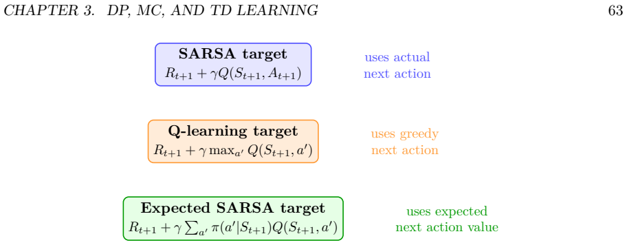
Figure 3.7. Figure 3.7: SARSA, Q-learning, and Expected SARSA differ mainly in the bootstrap target. [PITH_FULL_IMAGE:figures/full_fig_p066_3_7.png] view at source ↗
Figure 3.8
Figure 3.8. Figure 3.8: Eligibility traces assign credit backward through recently visited states. The trace [PITH_FULL_IMAGE:figures/full_fig_p066_3_8.png] view at source ↗
Figure 3.9
Figure 3.9. Figure 3.9: Conceptual map of classical value-learning methods. DP, MC, TD, multi-step TD, [PITH_FULL_IMAGE:figures/full_fig_p067_3_9.png] view at source ↗
Figure 3.10
Figure 3.10. Figure 3.10: Example grid-world. Walls block movement, the start state is marked S, and the [PITH_FULL_IMAGE:figures/full_fig_p073_3_10.png] view at source ↗
Figure 3.11
Figure 3.11. Figure 3.11: Interpretation of TD learning for UAV-assisted network control. A transition [PITH_FULL_IMAGE:figures/full_fig_p074_3_11.png] view at source ↗
Figure 4.1
Figure 4.1. Figure 4.1: Chapter 4 is the bridge from classical RL to deep RL. The mathematical update [PITH_FULL_IMAGE:figures/full_fig_p081_4_1.png] view at source ↗
Figure 4.2
Figure 4.2. Figure 4.2: A table stores separate values for separate state-action pairs. A function approximator [PITH_FULL_IMAGE:figures/full_fig_p082_4_2.png] view at source ↗
Figure 4.3
Figure 4.3. Figure 4.3: The curse of dimensionality. Even coarse discretization becomes impossible as the [PITH_FULL_IMAGE:figures/full_fig_p083_4_3.png] view at source ↗
Figure 4.4
Figure 4.4. Figure 4.4: High-dimensional observations require representation learning. Deep RL uses neural [PITH_FULL_IMAGE:figures/full_fig_p084_4_4.png] view at source ↗
Figure 4.5
Figure 4.5. Figure 4.5: Generalization allows learning from similar states. In a table, unseen states have [PITH_FULL_IMAGE:figures/full_fig_p084_4_5.png] view at source ↗
Figure 4.6
Figure 4.6. Figure 4.6: Feature-based value approximation. The designer chooses [PITH_FULL_IMAGE:figures/full_fig_p086_4_6.png] view at source ↗
Figure 4.7
Figure 4.7. Figure 4.7: Fitted value iteration turns RL into repeated supervised regression. The difficulty [PITH_FULL_IMAGE:figures/full_fig_p087_4_7.png] view at source ↗
Figure 4.8
Figure 4.8. Figure 4.8: DQN was built on a long chain of ideas: replay, function approximation, warnings [PITH_FULL_IMAGE:figures/full_fig_p088_4_8.png] view at source ↗
Figure 4.9
Figure 4.9. Figure 4.9: The moving-target problem in deep RL. The policy determines data, the data [PITH_FULL_IMAGE:figures/full_fig_p089_4_9.png] view at source ↗
Figure 4.10
Figure 4.10. Figure 4.10: The deadly triad: function approximation, bootstrapping, and off-policy learning. [PITH_FULL_IMAGE:figures/full_fig_p090_4_10.png] view at source ↗
Figure 4.11
Figure 4.11. Figure 4.11: Replay and target networks stabilize deep value learning. Replay improves data [PITH_FULL_IMAGE:figures/full_fig_p091_4_11.png] view at source ↗
Figure 4.12
Figure 4.12. Figure 4.12: In UAV network control, the state is naturally structured and high-dimensional. [PITH_FULL_IMAGE:figures/full_fig_p092_4_12.png] view at source ↗
Figure 4.13
Figure 4.13. Figure 4.13: A neural Q-function for discrete actions. The input is a feature vector or encoded [PITH_FULL_IMAGE:figures/full_fig_p093_4_13.png] view at source ↗
Figure 4.14
Figure 4.14. Figure 4.14: Conceptual route to DQN. DQN is not merely neural Q-learning; it is neural [PITH_FULL_IMAGE:figures/full_fig_p096_4_14.png] view at source ↗
Figure 5.1
Figure 5.1. Figure 5.1: DQN is not only a neural network. It is a training system that combines pixel [PITH_FULL_IMAGE:figures/full_fig_p101_5_1.png] view at source ↗
Figure 5.2
Figure 5.2. Figure 5.2: The Arcade Learning Environment turned Atari 2600 games into a common RL [PITH_FULL_IMAGE:figures/full_fig_p102_5_2.png] view at source ↗
Figure 5.3
Figure 5.3. Figure 5.3: DQN replaces the Q-table with a neural network. Instead of storing one value per [PITH_FULL_IMAGE:figures/full_fig_p103_5_3.png] view at source ↗
Figure 5.4
Figure 5.4. Figure 5.4: DQN combines function approximation, bootstrapping, and off-policy learning. This [PITH_FULL_IMAGE:figures/full_fig_p104_5_4.png] view at source ↗
Figure 5.5
Figure 5.5. Figure 5.5: A simplified sketch of the intuition behind Baird’s counterexample. The exact feature [PITH_FULL_IMAGE:figures/full_fig_p105_5_5.png] view at source ↗
Figure 5.6
Figure 5.6. Figure 5.6: DQN is a closed-loop training system. The agent collects transitions, stores them in [PITH_FULL_IMAGE:figures/full_fig_p106_5_6.png] view at source ↗
Figure 5.7
Figure 5.7. Figure 5.7: Frame stacking gives the Q-network short-term memory. In many Atari games, one [PITH_FULL_IMAGE:figures/full_fig_p107_5_7.png] view at source ↗
Figure 5.8
Figure 5.8. Figure 5.8: The DQN architecture maps stacked preprocessed frames to a vector of action values. [PITH_FULL_IMAGE:figures/full_fig_p108_5_8.png] view at source ↗
Figure 5.9
Figure 5.9. Figure 5.9: Experience replay converts an online stream of correlated transitions into randomly [PITH_FULL_IMAGE:figures/full_fig_p109_5_9.png] view at source ↗
Figure 5.10
Figure 5.10. Figure 5.10: Experience replay reduces local temporal correlation by sampling from a buffer [PITH_FULL_IMAGE:figures/full_fig_p110_5_10.png] view at source ↗
Figure 5.11
Figure 5.11. Figure 5.11: The target network computes the bootstrap target using delayed parameters [PITH_FULL_IMAGE:figures/full_fig_p111_5_11.png] view at source ↗
Figure 5.12
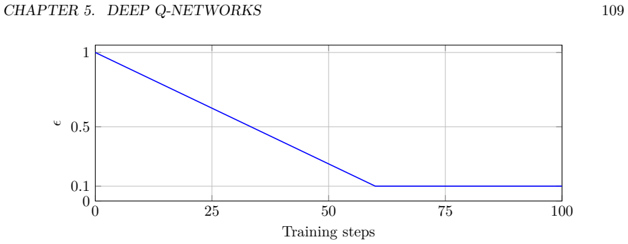
Figure 5.12. Figure 5.12: A typical epsilon schedule decreases exploration over training. Early exploration [PITH_FULL_IMAGE:figures/full_fig_p112_5_12.png] view at source ↗
Figure 5.13
Figure 5.13. Figure 5.13: A debugging map for DQN. Training failure can come from many sources: incorrect [PITH_FULL_IMAGE:figures/full_fig_p119_5_13.png] view at source ↗
Figure 5.14
Figure 5.14. Figure 5.14: DQN opened a family of value-based deep RL algorithms. Many later methods can [PITH_FULL_IMAGE:figures/full_fig_p120_5_14.png] view at source ↗
Figure 6.1
Figure 6.1. Figure 6.1: The DQN family can be understood as a set of targeted improvements. Each [PITH_FULL_IMAGE:figures/full_fig_p127_6_1.png] view at source ↗
Figure 6.2
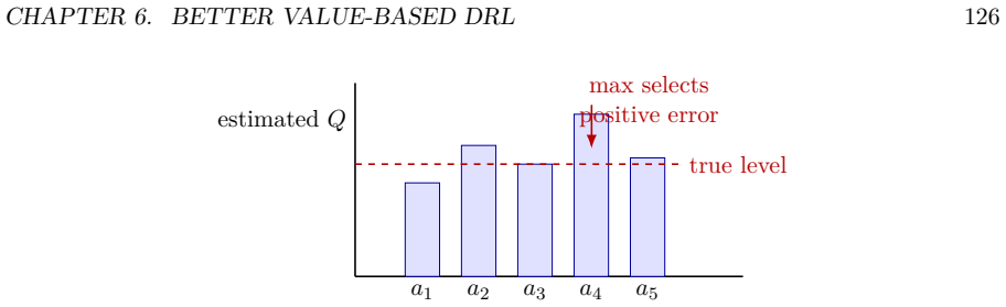
Figure 6.2. Figure 6.2: Overestimation bias arises because the maximum over noisy estimates tends to select [PITH_FULL_IMAGE:figures/full_fig_p129_6_2.png] view at source ↗
Figure 6.3
Figure 6.3. Figure 6.3: Double DQN decouples selection and evaluation. The online network chooses the [PITH_FULL_IMAGE:figures/full_fig_p129_6_3.png] view at source ↗
Figure 6.4
Figure 6.4. Figure 6.4: The dueling architecture estimates state value and action advantage using separate [PITH_FULL_IMAGE:figures/full_fig_p130_6_4.png] view at source ↗
Figure 6.5
Figure 6.5. Figure 6.5: Prioritized replay samples transitions with probability related to their learning [PITH_FULL_IMAGE:figures/full_fig_p131_6_5.png] view at source ↗
Figure 6.6
Figure 6.6. Figure 6.6: Multi-step targets combine sampled rewards over several steps with a later bootstrap [PITH_FULL_IMAGE:figures/full_fig_p131_6_6.png] view at source ↗
Figure 6.7
Figure 6.7. Figure 6.7: Noisy networks inject learned parameter-space noise into value networks. This [PITH_FULL_IMAGE:figures/full_fig_p132_6_7.png] view at source ↗
Figure 6.8
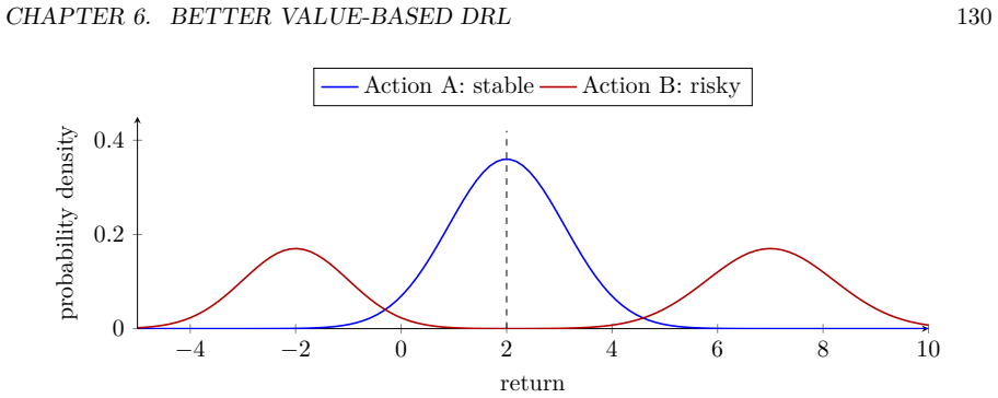
Figure 6.8. Figure 6.8: Two actions can have similar expected return but very different return distributions. [PITH_FULL_IMAGE:figures/full_fig_p133_6_8.png] view at source ↗
Figure 6.9
Figure 6.9. Figure 6.9: C51 represents the return distribution using fixed atoms. The target distribution is [PITH_FULL_IMAGE:figures/full_fig_p134_6_9.png] view at source ↗
Figure 6.10
Figure 6.10. Figure 6.10: Quantile distributional methods represent return distributions through quantile [PITH_FULL_IMAGE:figures/full_fig_p134_6_10.png] view at source ↗
Figure 6.11
Figure 6.11. Figure 6.11: Rainbow DQN combines several complementary improvements. Its value is not [PITH_FULL_IMAGE:figures/full_fig_p135_6_11.png] view at source ↗
Figure 6.12
Figure 6.12. Figure 6.12: In UAV/SDN control, the DQN-family mechanisms have concrete interpretations. [PITH_FULL_IMAGE:figures/full_fig_p137_6_12.png] view at source ↗
Figure 7.1
Figure 7.1. Figure 7.1: Value-based methods learn action values and derive behavior via [PITH_FULL_IMAGE:figures/full_fig_p149_7_1.png] view at source ↗
Figure 7.2
Figure 7.2. Figure 7.2: Discretizing continuous action spaces creates exponential growth in the number of [PITH_FULL_IMAGE:figures/full_fig_p151_7_2.png] view at source ↗
Figure 7.3
Figure 7.3. Figure 7.3: A neural policy can output the parameters of an action distribution. For continuous [PITH_FULL_IMAGE:figures/full_fig_p151_7_3.png] view at source ↗
Figure 7.4
Figure 7.4. Figure 7.4: A trajectory distribution depends on both the policy and the environment dynamics. [PITH_FULL_IMAGE:figures/full_fig_p152_7_4.png] view at source ↗
Figure 7.5
Figure 7.5. Figure 7.5: The likelihood-ratio estimator multiplies a score term by a return estimate. The [PITH_FULL_IMAGE:figures/full_fig_p153_7_5.png] view at source ↗
Figure 7.6
Figure 7.6. Figure 7.6: The policy-gradient theorem separates the gradient into two conceptual parts: a [PITH_FULL_IMAGE:figures/full_fig_p154_7_6.png] view at source ↗
Figure 7.7
Figure 7.7. Figure 7.7: For a continuous Gaussian policy, a policy-gradient update can shift the mean and [PITH_FULL_IMAGE:figures/full_fig_p155_7_7.png] view at source ↗
Figure 7.8
Figure 7.8. Figure 7.8: A structured policy can factorize a complex decision into a discrete mode and [PITH_FULL_IMAGE:figures/full_fig_p158_7_8.png] view at source ↗
Figure 7.9
Figure 7.9. Figure 7.9: Policy gradients form the foundation for many later algorithms. REINFORCE [PITH_FULL_IMAGE:figures/full_fig_p158_7_9.png] view at source ↗
Figure 7.10
Figure 7.10. Figure 7.10: A direct policy-gradient architecture for UAV/SDN control can use multiple policy [PITH_FULL_IMAGE:figures/full_fig_p160_7_10.png] view at source ↗
Figure 8.1
Figure 8.1. Figure 8.1: The policy-gradient pipeline. REINFORCE begins with sampled trajectories and [PITH_FULL_IMAGE:figures/full_fig_p170_8_1.png] view at source ↗
Figure 8.2
Figure 8.2. Figure 8.2: Full-return credit assignment. A single trajectory return gives a coarse learning [PITH_FULL_IMAGE:figures/full_fig_p172_8_2.png] view at source ↗
Figure 8.3
Figure 8.3. Figure 8.3: The causality trick. The action at time t can affect future rewards but not past rewards. Reward-to-go therefore reduces variance without changing the expected gradient. return b(s) Raw signal Gt Centered signal Gt − b(s) Subtracting a baseline recenters the learning signal around what was expected. Positive values mean better than expected; negative values mean worse than expected [PITH_FULL_IMAGE:figu… view at source ↗
Figure 8.4
Figure 8.4. Figure 8.4: A baseline acts like a control variate. It can center the return distribution and reduce [PITH_FULL_IMAGE:figures/full_fig_p173_8_4.png] view at source ↗
Figure 8.5
Figure 8.5. Figure 8.5: Advantage as relative action quality. The baseline [PITH_FULL_IMAGE:figures/full_fig_p174_8_5.png] view at source ↗
Figure 8.6
Figure 8.6. Figure 8.6: Advantage estimators trade bias against variance. GAE provides a smooth interpola [PITH_FULL_IMAGE:figures/full_fig_p176_8_6.png] view at source ↗
Figure 8.7
Figure 8.7. Figure 8.7: Advantage-based policy update in a UAV/SDN control state. The policy is not [PITH_FULL_IMAGE:figures/full_fig_p181_8_7.png] view at source ↗
Figure 8.8
Figure 8.8. Figure 8.8: REINFORCE-style advantage estimation for language-model RL. RLOO and GRPO [PITH_FULL_IMAGE:figures/full_fig_p183_8_8.png] view at source ↗
Figure 9.1
Figure 9.1. Figure 9.1: The actor-critic idea. The actor chooses actions. The critic evaluates the consequences [PITH_FULL_IMAGE:figures/full_fig_p187_9_1.png] view at source ↗
Figure 9.2
Figure 9.2. Figure 9.2: From REINFORCE to actor-critic. Actor-critic methods replace raw Monte Carlo [PITH_FULL_IMAGE:figures/full_fig_p189_9_2.png] view at source ↗
Figure 9.3
Figure 9.3. Figure 9.3: Different critics support different actor-critic families. On-policy methods often [PITH_FULL_IMAGE:figures/full_fig_p190_9_3.png] view at source ↗
Figure 9.4
Figure 9.4. Figure 9.4: Actor-critic target choices. One-step TD has low variance but can be biased by [PITH_FULL_IMAGE:figures/full_fig_p190_9_4.png] view at source ↗
Figure 9.5
Figure 9.5. Figure 9.5: A2C and A3C use multiple actor-learners. A3C performs asynchronous updates, [PITH_FULL_IMAGE:figures/full_fig_p191_9_5.png] view at source ↗
Figure 9.6
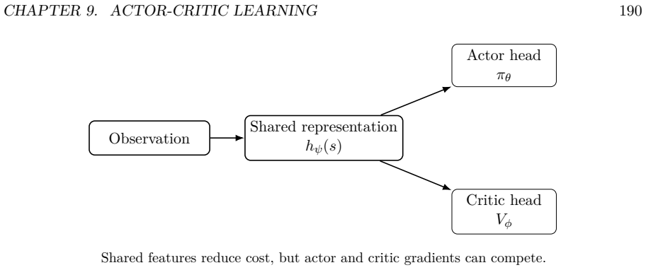
Figure 9.6. Figure 9.6: Shared actor-critic networks. A shared trunk can be efficient, but actor and critic [PITH_FULL_IMAGE:figures/full_fig_p193_9_6.png] view at source ↗
Figure 9.7
Figure 9.7. Figure 9.7: Off-policy actor-critic. Data may be generated by a behavior policy different from [PITH_FULL_IMAGE:figures/full_fig_p194_9_7.png] view at source ↗
Figure 9.8
Figure 9.8. Figure 9.8: Deterministic actor-critic. The critic is differentiable with respect to the action, so [PITH_FULL_IMAGE:figures/full_fig_p194_9_8.png] view at source ↗
Figure 9.9
Figure 9.9. Figure 9.9: A UAV/SDN actor–critic architecture. The actor proposes continuous control actions; [PITH_FULL_IMAGE:figures/full_fig_p197_9_9.png] view at source ↗
Figure 10.1
Figure 10.1. Figure 10.1: PPO alternates between collecting on-policy data, estimating advantages, and [PITH_FULL_IMAGE:figures/full_fig_p205_10_1.png] view at source ↗
Figure 10.2
Figure 10.2. Figure 10.2: PPO can be understood as a practical approximation to the trust-region idea. [PITH_FULL_IMAGE:figures/full_fig_p206_10_2.png] view at source ↗
Figure 10.3
Figure 10.3. Figure 10.3: The PPO clipped surrogate for positive and negative advantages when [PITH_FULL_IMAGE:figures/full_fig_p207_10_3.png] view at source ↗
Figure 10.4
Figure 10.4. Figure 10.4: PPO is usually implemented as an actor-critic method. The actor uses the clipped [PITH_FULL_IMAGE:figures/full_fig_p208_10_4.png] view at source ↗
Figure 10.5
Figure 10.5. Figure 10.5: PPO should be monitored through multiple diagnostics, not only reward. Approxi [PITH_FULL_IMAGE:figures/full_fig_p215_10_5.png] view at source ↗
Figure 10.6
Figure 10.6. Figure 10.6: A PPO-style UAV/SDN control architecture. PPO proposes stochastic continuous [PITH_FULL_IMAGE:figures/full_fig_p215_10_6.png] view at source ↗
Figure 10.7
Figure 10.7. Figure 10.7: PPO-style RLHF for language models. A policy model samples completions, [PITH_FULL_IMAGE:figures/full_fig_p217_10_7.png] view at source ↗
Figure 11.1
Figure 11.1. Figure 11.1: Why SAC appears after PPO, DDPG, and TD3. PPO is robust but often sample [PITH_FULL_IMAGE:figures/full_fig_p221_11_1.png] view at source ↗
Figure 11.2
Figure 11.2. Figure 11.2: The soft Bellman backup. SAC changes the value target by subtracting the [PITH_FULL_IMAGE:figures/full_fig_p223_11_2.png] view at source ↗
Figure 11.3
Figure 11.3. Figure 11.3: The conceptual loop behind SAC. SAC learns critics, a stochastic actor, and often [PITH_FULL_IMAGE:figures/full_fig_p224_11_3.png] view at source ↗
Figure 11.4
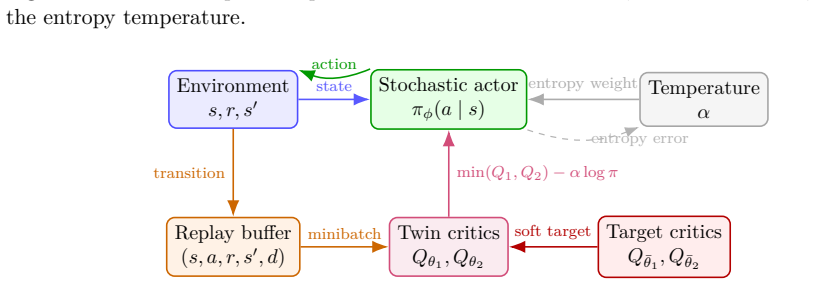
Figure 11.4. Figure 11.4: The SAC architecture. SAC stores environment transitions in a replay buffer, trains [PITH_FULL_IMAGE:figures/full_fig_p224_11_4.png] view at source ↗
Figure 11.5
Figure 11.5. Figure 11.5: The squashed Gaussian policy used in SAC. The Gaussian sample is differentiable [PITH_FULL_IMAGE:figures/full_fig_p225_11_5.png] view at source ↗
Figure 11.6
Figure 11.6. Figure 11.6: Automatic entropy-temperature tuning. SAC adapts [PITH_FULL_IMAGE:figures/full_fig_p226_11_6.png] view at source ↗
Figure 11.7
Figure 11.7. Figure 11.7: SAC for UAV/SDN control. The actor proposes stochastic continuous actions, [PITH_FULL_IMAGE:figures/full_fig_p232_11_7.png] view at source ↗
Figure 12.1
Figure 12.1. Figure 12.1: The central loop of model-based reinforcement learning. Real interaction trains [PITH_FULL_IMAGE:figures/full_fig_p238_12_1.png] view at source ↗
Figure 12.2
Figure 12.2. Figure 12.2: Model-free and model-based learning. Model-free methods update the policy or [PITH_FULL_IMAGE:figures/full_fig_p240_12_2.png] view at source ↗
Figure 12.3
Figure 12.3. Figure 12.3: The Dyna architecture. The agent learns from real experience and from model [PITH_FULL_IMAGE:figures/full_fig_p240_12_3.png] view at source ↗
Figure 12.4
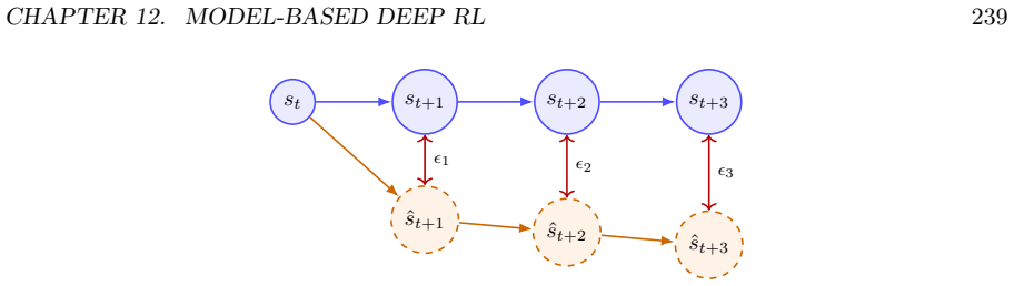
Figure 12.4. Figure 12.4: Compounding model error. A small one-step prediction error can grow when model [PITH_FULL_IMAGE:figures/full_fig_p242_12_4.png] view at source ↗
Figure 12.5
Figure 12.5. Figure 12.5: Ensemble uncertainty. Multiple learned models predict the next state or latent [PITH_FULL_IMAGE:figures/full_fig_p242_12_5.png] view at source ↗
Figure 12.6
Figure 12.6. Figure 12.6: MBPO-style short-horizon rollouts. The learned model is used only for short [PITH_FULL_IMAGE:figures/full_fig_p244_12_6.png] view at source ↗
Figure 12.7
Figure 12.7. Figure 12.7: CEM planning for model-predictive control. The planner samples action sequences, [PITH_FULL_IMAGE:figures/full_fig_p245_12_7.png] view at source ↗
Figure 12.8
Figure 12.8. Figure 12.8: A latent world model. Observations are encoded into a latent state. The model [PITH_FULL_IMAGE:figures/full_fig_p246_12_8.png] view at source ↗
Figure 12.9
Figure 12.9. Figure 12.9: Dreamer-style imagination learning. The world model is trained from real data. [PITH_FULL_IMAGE:figures/full_fig_p247_12_9.png] view at source ↗
Figure 12.10
Figure 12.10. Figure 12.10: MuZero-style value-equivalent modeling. The model predicts the quantities needed [PITH_FULL_IMAGE:figures/full_fig_p248_12_10.png] view at source ↗
Figure 12.11
Figure 12.11. Figure 12.11: TD-MPC-style latent planning. The model predicts control-relevant quantities in [PITH_FULL_IMAGE:figures/full_fig_p248_12_11.png] view at source ↗
Figure 12.12
Figure 12.12. Figure 12.12: Model-based UAV/SDN control. A learned network model predicts future QoS [PITH_FULL_IMAGE:figures/full_fig_p249_12_12.png] view at source ↗
Figure 13.1
Figure 13.1. Figure 13.1: The historical arc from AlphaZero to MuZero-style agents. AlphaZero uses search [PITH_FULL_IMAGE:figures/full_fig_p256_13_1.png] view at source ↗
Figure 13.2
Figure 13.2. Figure 13.2: The MuZero network decomposition. The representation function initializes a latent [PITH_FULL_IMAGE:figures/full_fig_p258_13_2.png] view at source ↗
Figure 13.3
Figure 13.3. Figure 13.3: MuZero plans in a learned latent state space. Search does not require a perfect [PITH_FULL_IMAGE:figures/full_fig_p259_13_3.png] view at source ↗
Figure 13.4
Figure 13.4. Figure 13.4: MuZero training unroll. The learned dynamics model is unrolled through real [PITH_FULL_IMAGE:figures/full_fig_p260_13_4.png] view at source ↗
Figure 13.5
Figure 13.5. Figure 13.5: A MuZero-style UAV/SDN control scenario. The agent maps telemetry into a [PITH_FULL_IMAGE:figures/full_fig_p267_13_5.png] view at source ↗
Figure 14.1
Figure 14.1. Figure 14.1: Online RL learns through interaction; offline RL learns from a fixed dataset. Offline [PITH_FULL_IMAGE:figures/full_fig_p273_14_1.png] view at source ↗
Figure 14.2
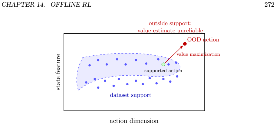
Figure 14.2. Figure 14.2: Offline RL must avoid unsupported state–action regions. The blue points represent [PITH_FULL_IMAGE:figures/full_fig_p275_14_2.png] view at source ↗
Figure 14.3
Figure 14.3. Figure 14.3: Extrapolation error in offline Q-learning. The value maximization step may select [PITH_FULL_IMAGE:figures/full_fig_p276_14_3.png] view at source ↗
Figure 14.4
Figure 14.4. Figure 14.4: CQL adds pessimism to the critic. Unsupported actions are penalized so that value [PITH_FULL_IMAGE:figures/full_fig_p278_14_4.png] view at source ↗
Figure 14.5
Figure 14.5. Figure 14.5: Decision Transformer treats offline RL as return-conditioned sequence modeling. [PITH_FULL_IMAGE:figures/full_fig_p280_14_5.png] view at source ↗
Figure 14.6
Figure 14.6. Figure 14.6: Offline RL for UAV/SDN control. Historical network logs are converted into an [PITH_FULL_IMAGE:figures/full_fig_p283_14_6.png] view at source ↗
Figure 15.1
Figure 15.1. Figure 15.1: Decision Transformer views a trajectory as a token sequence of return-to-go, state, [PITH_FULL_IMAGE:figures/full_fig_p291_15_1.png] view at source ↗
Figure 15.2
Figure 15.2. Figure 15.2: Decision Transformer architecture. Return-to-go, state, and action tokens are [PITH_FULL_IMAGE:figures/full_fig_p293_15_2.png] view at source ↗
Figure 15.3
Figure 15.3. Figure 15.3: Decision Transformer inference. A target return conditions the policy. After each [PITH_FULL_IMAGE:figures/full_fig_p293_15_3.png] view at source ↗
Figure 15.4
Figure 15.4. Figure 15.4: Decision Transformer and Trajectory Transformer both use sequence modeling, but [PITH_FULL_IMAGE:figures/full_fig_p298_15_4.png] view at source ↗
Figure 15.5
Figure 15.5. Figure 15.5: Trajectory stitching. Two suboptimal dataset trajectories may contain useful [PITH_FULL_IMAGE:figures/full_fig_p299_15_5.png] view at source ↗
Figure 15.6
Figure 15.6. Figure 15.6: A Decision Transformer scenario for UAV/SDN control. Historical network logs are [PITH_FULL_IMAGE:figures/full_fig_p301_15_6.png] view at source ↗
Figure 16.1
Figure 16.1. Figure 16.1: The transition from single-agent RL to multi-agent RL. Adding agents creates new [PITH_FULL_IMAGE:figures/full_fig_p308_16_1.png] view at source ↗
Figure 16.2
Figure 16.2. Figure 16.2: A Dec-POMDP view of cooperative MARL. The environment has a global state, [PITH_FULL_IMAGE:figures/full_fig_p309_16_2.png] view at source ↗
Figure 16.3
Figure 16.3. Figure 16.3: Independent learners face non-stationarity. Each agent updates its own policy, [PITH_FULL_IMAGE:figures/full_fig_p311_16_3.png] view at source ↗
Figure 16.4
Figure 16.4. Figure 16.4: Centralized training with decentralized execution. The training process may use [PITH_FULL_IMAGE:figures/full_fig_p312_16_4.png] view at source ↗
Figure 16.5
Figure 16.5. Figure 16.5: The QMIX idea. Per-agent utilities are combined by a monotonic mixer conditioned [PITH_FULL_IMAGE:figures/full_fig_p313_16_5.png] view at source ↗
Figure 16.6
Figure 16.6. Figure 16.6: Centralized-critic actor-critic MARL. Decentralized actors choose actions from [PITH_FULL_IMAGE:figures/full_fig_p315_16_6.png] view at source ↗
Figure 16.7
Figure 16.7. Figure 16.7: A graph view of MARL. Each agent is a node, and edges represent communication, [PITH_FULL_IMAGE:figures/full_fig_p316_16_7.png] view at source ↗
Figure 16.8
Figure 16.8. Figure 16.8: A multi-agent UAV/SDN scenario. UAVs coordinate movement, spectrum allocation, [PITH_FULL_IMAGE:figures/full_fig_p318_16_8.png] view at source ↗
Figure 17.1
Figure 17.1. Figure 17.1: The basic two-level HRL architecture. A high-level policy chooses a temporally [PITH_FULL_IMAGE:figures/full_fig_p328_17_1.png] view at source ↗
Figure 17.2
Figure 17.2. Figure 17.2: In an SMDP, a temporally extended option can last for multiple primitive steps. The [PITH_FULL_IMAGE:figures/full_fig_p330_17_2.png] view at source ↗
Figure 17.3
Figure 17.3. Figure 17.3: The three components of an option: initiation set, intra-option policy, and termina [PITH_FULL_IMAGE:figures/full_fig_p330_17_3.png] view at source ↗
Figure 17.4
Figure 17.4. Figure 17.4: Option-Critic learns intra-option policies and termination functions. A termination [PITH_FULL_IMAGE:figures/full_fig_p332_17_4.png] view at source ↗
Figure 17.5
Figure 17.5. Figure 17.5: Unsupervised skill discovery learns a latent-conditioned policy whose behaviors are [PITH_FULL_IMAGE:figures/full_fig_p334_17_5.png] view at source ↗
Figure 17.6
Figure 17.6. Figure 17.6: Event-conditioned HRL for UAV/SDN control. High-level mission modes are [PITH_FULL_IMAGE:figures/full_fig_p335_17_6.png] view at source ↗
Figure 18.1
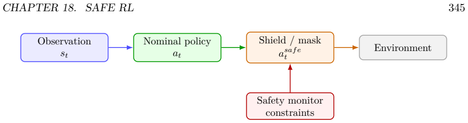
Figure 18.1. Figure 18.1: Safe RL extends reward maximization with explicit constraints. The policy must [PITH_FULL_IMAGE:figures/full_fig_p343_18_1.png] view at source ↗
Figure 18.2
Figure 18.2. Figure 18.2: A CMDP separates reward from cost. Reward measures task performance, while [PITH_FULL_IMAGE:figures/full_fig_p345_18_2.png] view at source ↗
Figure 18.3
Figure 18.3. Figure 18.3: Primal-dual safe RL. The actor optimizes a reward-cost trade-off, while the Lagrange [PITH_FULL_IMAGE:figures/full_fig_p346_18_3.png] view at source ↗
Figure 18.4
Figure 18.4. Figure 18.4: Shielded RL. The policy proposes an action, but a safety module masks, rejects, or [PITH_FULL_IMAGE:figures/full_fig_p348_18_4.png] view at source ↗
Figure 18.5
Figure 18.5. Figure 18.5: CBF safety filtering. A nominal RL action may point outside the safe set; the [PITH_FULL_IMAGE:figures/full_fig_p349_18_5.png] view at source ↗
Figure 18.6
Figure 18.6. Figure 18.6: A safe UAV/SDN actor-critic architecture. The actor proposes resource and [PITH_FULL_IMAGE:figures/full_fig_p351_18_6.png] view at source ↗
Figure 19.1
Figure 19.1. Figure 19.1: Preference learning turns human judgment into a reward-learning problem. The [PITH_FULL_IMAGE:figures/full_fig_p362_19_1.png] view at source ↗
Figure 19.2
Figure 19.2. Figure 19.2: The canonical RLHF pipeline. A pretrained model is instruction-tuned, a reward [PITH_FULL_IMAGE:figures/full_fig_p362_19_2.png] view at source ↗
Figure 19.3
Figure 19.3. Figure 19.3: Reward-model training with a pairwise preference loss. The model learns to assign [PITH_FULL_IMAGE:figures/full_fig_p364_19_3.png] view at source ↗
Figure 19.4
Figure 19.4. Figure 19.4: PPO-style RLHF. The policy samples responses, the reward model scores them, the [PITH_FULL_IMAGE:figures/full_fig_p365_19_4.png] view at source ↗
Figure 19.5
Figure 19.5. Figure 19.5: Reward-model overoptimization. As optimization strength increases, the learned [PITH_FULL_IMAGE:figures/full_fig_p365_19_5.png] view at source ↗
Figure 19.6
Figure 19.6. Figure 19.6: Two broad post-training paths from preference data. RLHF trains a reward model [PITH_FULL_IMAGE:figures/full_fig_p367_19_6.png] view at source ↗
Figure 19.7
Figure 19.7. Figure 19.7: A technical RLHF scenario. Human operators compare alternative network [PITH_FULL_IMAGE:figures/full_fig_p368_19_7.png] view at source ↗
Figure 20.1
Figure 20.1. Figure 20.1: Reasoning as reinforcement learning. A model generates a reasoning trajectory; a [PITH_FULL_IMAGE:figures/full_fig_p378_20_1.png] view at source ↗
Figure 20.2
Figure 20.2. Figure 20.2: Outcome rewards supervise the final answer; process rewards supervise intermediate [PITH_FULL_IMAGE:figures/full_fig_p379_20_2.png] view at source ↗
Figure 20.3
Figure 20.3. Figure 20.3: Group-relative reasoning RL. Multiple completions for the same prompt are scored [PITH_FULL_IMAGE:figures/full_fig_p381_20_3.png] view at source ↗
Figure 20.4
Figure 20.4. Figure 20.4: Outcome-level reasoning reward creates long-horizon credit assignment. The final [PITH_FULL_IMAGE:figures/full_fig_p382_20_4.png] view at source ↗
Figure 20.5
Figure 20.5. Figure 20.5: Inference-time scaling for reasoning. The model samples or searches over multiple [PITH_FULL_IMAGE:figures/full_fig_p384_20_5.png] view at source ↗
Figure 20.6
Figure 20.6. Figure 20.6: A reasoning-RL assistant for SD-WAN/UAV control. The reasoning model proposes [PITH_FULL_IMAGE:figures/full_fig_p385_20_6.png] view at source ↗
Figure 20.7
Figure 20.7. Figure 20.7: A practical reasoning-RL pipeline. Reasoning ability is improved by generating [PITH_FULL_IMAGE:figures/full_fig_p386_20_7.png] view at source ↗
Figure 21.1
Figure 21.1. Figure 21.1: Network DRL must be matched to the control timescale. A packet-level controller [PITH_FULL_IMAGE:figures/full_fig_p398_21_1.png] view at source ↗
Figure 21.2
Figure 21.2. Figure 21.2: Network state is an engineered object. The observation used by a DRL agent is the [PITH_FULL_IMAGE:figures/full_fig_p400_21_2.png] view at source ↗
Figure 21.3
Figure 21.3. Figure 21.3: A closed-loop DRL architecture for networks. In deployment, the learned policy [PITH_FULL_IMAGE:figures/full_fig_p401_21_3.png] view at source ↗
Figure 21.4
Figure 21.4. Figure 21.4: SD-WAN traffic engineering as a safe DRL problem. The actor proposes traffic [PITH_FULL_IMAGE:figures/full_fig_p403_21_4.png] view at source ↗
Figure 21.5
Figure 21.5. Figure 21.5: A multi-UAV network-slicing scenario. UAVs provide aerial connectivity to [PITH_FULL_IMAGE:figures/full_fig_p404_21_5.png] view at source ↗
Figure 21.6
Figure 21.6. Figure 21.6: A simulator-in-the-loop network DRL pipeline. Credible work does not stop at [PITH_FULL_IMAGE:figures/full_fig_p405_21_6.png] view at source ↗
Figure 21.7
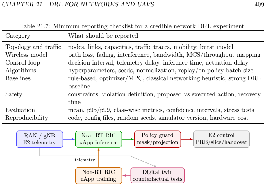
Figure 21.7. Figure 21.7: A practical O-RAN DRL blueprint. Fast inference and safety guards belong near [PITH_FULL_IMAGE:figures/full_fig_p412_21_7.png] view at source ↗
Figure 21.8
Figure 21.8. Figure 21.8: Deployment gates for network DRL. A policy should not move directly from [PITH_FULL_IMAGE:figures/full_fig_p416_21_8.png] view at source ↗
Figure 22.1
Figure 22.1. Figure 22.1: A research-grade DRL implementation pipeline. A serious project must connect [PITH_FULL_IMAGE:figures/full_fig_p423_22_1.png] view at source ↗
Figure 22.2
Figure 22.2. Figure 22.2: Scenario-first implementation for safe UAV/SD-WAN control. The policy is only one [PITH_FULL_IMAGE:figures/full_fig_p423_22_2.png] view at source ↗
Figure 22.3
Figure 22.3. Figure 22.3: The environment contract. The observation, action, reward, termination flags, and [PITH_FULL_IMAGE:figures/full_fig_p426_22_3.png] view at source ↗
Figure 22.4
Figure 22.4. Figure 22.4: Training-loop architecture. The data path and artifact path should be explicit: [PITH_FULL_IMAGE:figures/full_fig_p432_22_4.png] view at source ↗
Figure 22.5
Figure 22.5. Figure 22.5: Ablation design. A credible DRL paper should isolate the contribution of each [PITH_FULL_IMAGE:figures/full_fig_p436_22_5.png] view at source ↗
Figure 22.6
Figure 22.6. Figure 22.6: Deployment gate for DRL systems. The model should pass offline tests, stress tests, [PITH_FULL_IMAGE:figures/full_fig_p439_22_6.png] view at source ↗
Figure 22.7
Figure 22.7. Figure 22.7: End-to-end implementation scenario for safe DRL in UAV/SD-WAN control. The [PITH_FULL_IMAGE:figures/full_fig_p440_22_7.png] view at source ↗
Figure 22.8
Figure 22.8. Figure 22.8: Failure triage for DRL systems. Most failures should be diagnosed by environment [PITH_FULL_IMAGE:figures/full_fig_p441_22_8.png] view at source ↗
Figure 23.1
Figure 23.1. Figure 23.1: A research-grade DRL experiment begins with a precise claim and turns that claim [PITH_FULL_IMAGE:figures/full_fig_p445_23_1.png] view at source ↗
Figure 23.2
Figure 23.2. Figure 23.2: Seed variance is not noise to be hidden; it is part of the result. A method that wins [PITH_FULL_IMAGE:figures/full_fig_p447_23_2.png] view at source ↗
Figure 23.3
Figure 23.3. Figure 23.3: A performance profile shows the fraction of runs or tasks above each normalized [PITH_FULL_IMAGE:figures/full_fig_p449_23_3.png] view at source ↗
Figure 23.4
Figure 23.4. Figure 23.4: Learning curves answer a different question from final performance. A method can [PITH_FULL_IMAGE:figures/full_fig_p452_23_4.png] view at source ↗
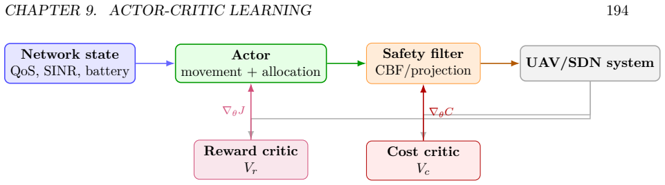
Figure 23.5
Figure 23.5. Figure 23.5: A serious DRL evaluation separates the reward used for training from the metrics [PITH_FULL_IMAGE:figures/full_fig_p453_23_5.png] view at source ↗
Figure 23.6
Figure 23.6. Figure 23.6: An ablation is a controlled experiment. Remove one component at a time and [PITH_FULL_IMAGE:figures/full_fig_p456_23_6.png] view at source ↗
Figure 23.7
Figure 23.7. Figure 23.7: Experimental methodology for a safe UAV/SD-WAN controller. Evaluation logs [PITH_FULL_IMAGE:figures/full_fig_p463_23_7.png] view at source ↗
Figure 24.1
Figure 24.1. Figure 24.1: A layered taxonomy of DRL failure modes. The same symptom, such as unstable [PITH_FULL_IMAGE:figures/full_fig_p469_24_1.png] view at source ↗
Figure 24.2
Figure 24.2. Figure 24.2: Reward hacking as proxy-objective exploitation. The policy optimizes the reward [PITH_FULL_IMAGE:figures/full_fig_p470_24_2.png] view at source ↗
Figure 24.3
Figure 24.3. Figure 24.3: The proposed-action versus executed-action failure. If a safety layer modifies [PITH_FULL_IMAGE:figures/full_fig_p474_24_3.png] view at source ↗
Figure 24.4
Figure 24.4. Figure 24.4: A practical DRL debugging pipeline. Algorithm tuning should come after environ [PITH_FULL_IMAGE:figures/full_fig_p480_24_4.png] view at source ↗
Figure 24.5
Figure 24.5. Figure 24.5: Failure analysis for safe SD-WAN traffic engineering. The audit must inspect reward, [PITH_FULL_IMAGE:figures/full_fig_p483_24_5.png] view at source ↗
Figure 25.1
Figure 25.1. Figure 25.1: A 2026 map of deep reinforcement learning. The field is moving from isolated [PITH_FULL_IMAGE:figures/full_fig_p488_25_1.png] view at source ↗
Figure 25.2
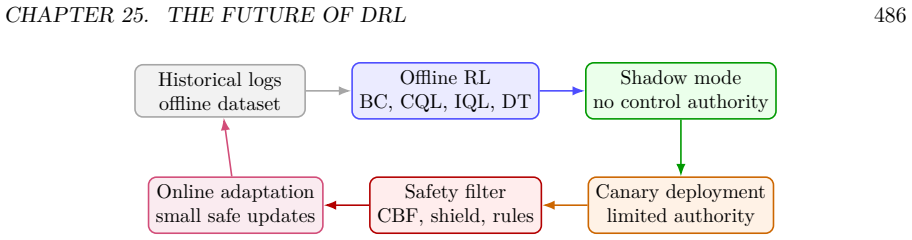
Figure 25.2. Figure 25.2: Offline-to-online reinforcement learning as a deployment lifecycle. Future systems [PITH_FULL_IMAGE:figures/full_fig_p489_25_2.png] view at source ↗
Figure 25.3
Figure 25.3. Figure 25.3: A unified future DRL stack. The policy is embedded inside a larger system [PITH_FULL_IMAGE:figures/full_fig_p492_25_3.png] view at source ↗
Figure 25.4
Figure 25.4. Figure 25.4: Future safe DRL scenario for UAV/SD-WAN control. A policy proposes actions, [PITH_FULL_IMAGE:figures/full_fig_p493_25_4.png] view at source ↗
Figure 25.5
Figure 25.5. Figure 25.5: A pragmatic research agenda after 2026. The field must first improve evaluation [PITH_FULL_IMAGE:figures/full_fig_p494_25_5.png] view at source ↗

discussion (0)

Sign in with ORCID, Apple, or X to comment. Anyone can read and Pith papers without signing in.

Reference graph

Works this paper leans on

51 extracted references · 44 linked inside Pith

  1. [7]

    Genie: Generative interactive environments

    Jake Bruce, Michael Dennis, Adam Edwards, et al. Genie: Generative interactive environments. arXiv preprint arXiv:2402.15391,

  2. [9]

    Soft actor-critic for discrete action settings.arXiv preprint arXiv:1910.07207,

    Petros Christodoulou. Soft actor-critic for discrete action settings.arXiv preprint arXiv:1910.07207,

  3. [14]

    D4RL: Datasets for deep data-driven reinforcement learning.arXiv preprint arXiv:2004.07219,

    Justin Fu, Aviral Kumar, Ofir Nachum, George Tucker, and Sergey Levine. D4RL: Datasets for deep data-driven reinforcement learning.arXiv preprint arXiv:2004.07219,

  4. [16]

    Improving alignment of dialogue agents via targeted human judgements.arXiv preprint arXiv:2209.14375,

    Amelia Glaese, Nat McAleese, et al. Improving alignment of dialogue agents via targeted human judgements.arXiv preprint arXiv:2209.14375,

  5. [17]

    Learning control barrier functions and their application in safe reinforcement learning.arXiv preprint arXiv:2404.16879,

    Maxime Guerrier, Hany Fouad, and Giovanni Beltrame. Learning control barrier functions and their application in safe reinforcement learning.arXiv preprint arXiv:2404.16879,

  6. [18]

    World models.arXiv preprint arXiv:1803.10122,

    David Ha and Jürgen Schmidhuber. World models.arXiv preprint arXiv:1803.10122,

  7. [19]

    Soft actor-critic: Off-policy maximum entropy deep reinforcement learning with a stochastic actor

    Tuomas Haarnoja, Aurick Zhou, Pieter Abbeel, and Sergey Levine. Soft actor-critic: Off-policy maximum entropy deep reinforcement learning with a stochastic actor. InInternational Conference on Machine Learning, 2018a. Tuomas Haarnoja, Aurick Zhou, Kristian Hartikainen, et al. Soft actor-critic algorithms and applications.arXiv preprint arXiv:1812.05905, 2...

  8. [20]

    Mastering diverse domains through world models.arXiv preprint arXiv:2301.04104,

    Danijar Hafner, Jurgis Pasukonis, Jimmy Ba, and Timothy Lillicrap. Mastering diverse domains through world models.arXiv preprint arXiv:2301.04104,

  9. [21]

    Nicklas Hansen, Xiaolong Wang, and Hao Su

    doi: 10.1038/s41586-025-08744-2. Nicklas Hansen, Xiaolong Wang, and Hao Su. Temporal difference learning for model predictive control. InInternational Conference on Machine Learning,

  10. [22]

    Dropout Q-functions for doubly efficient reinforcement learning.arXiv preprint arXiv:2110.02034,

    Takuya Hiraoka, Takuya Imagawa, Takuma Hashimoto, Takashi Onishi, and Yoshimasa Tsu- ruoka. Dropout Q-functions for doubly efficient reinforcement learning.arXiv preprint arXiv:2110.02034,

  11. [23]

    Orpo: Monolithic preference optimization without reference model.arXiv preprint arXiv:2403.07691,

    Jiwoo Hong, Noah Lee, and James Thorne. Orpo: Monolithic preference optimization without reference model.arXiv preprint arXiv:2403.07691,

  12. [24]

    A. U. Kaypak et al. A control barrier function-constrained model predictive control framework for safe reinforcement learning.arXiv preprint arXiv:2604.06463,

  13. [25]

    Kimi k1.5: Scaling reinforcement learning with LLMs.arXiv preprint arXiv:2501.12599,

    Kimi Team. Kimi k1.5: Scaling reinforcement learning with LLMs.arXiv preprint arXiv:2501.12599,

  14. [26]

    Kushwaha and Zachary A

    BIBLIOGRAPHY511 Deepak S. Kushwaha and Zachary A. Biron. A review on safe reinforcement learning using lyapunov and barrier functions.arXiv preprint arXiv:2508.09128,

  15. [28]

    Offline reinforcement learning: Tutorial, review, and perspectives on open problems.arXiv preprint arXiv:2005.01643,

    Sergey Levine, Aviral Kumar, George Tucker, and Justin Fu. Offline reinforcement learning: Tutorial, review, and perspectives on open problems.arXiv preprint arXiv:2005.01643,

  16. [29]

    Lillicrap, Jonathan J

    Timothy P. Lillicrap, Jonathan J. Hunt, Alexander Pritzel, et al. Continuous control with deep reinforcement learning.arXiv preprint arXiv:1509.02971,

  17. [30]

    Online finetuning decision transformers with pure reinforcement learning gradients.arXiv preprint arXiv:2601.00167,

    Junwei Luo and Yuke Zhu. Online finetuning decision transformers with pure reinforcement learning gradients.arXiv preprint arXiv:2601.00167,

  18. [31]

    Efficient soft actor-critic with LLM-based action-level guidance for continuous control.arXiv preprint arXiv:2603.17468,

    Huan Ma et al. Efficient soft actor-critic with LLM-based action-level guidance for continuous control.arXiv preprint arXiv:2603.17468,

  19. [32]

    SimPO: Simple preference optimization with a reference-free reward.arXiv preprint arXiv:2405.14734,

    Yu Meng, Mengzhou Xia, and Danqi Chen. SimPO: Simple preference optimization with a reference-free reward.arXiv preprint arXiv:2405.14734,

  20. [34]

    Accelerating online reinforce- ment learning with offline datasets.arXiv preprint arXiv:2006.09359,

    Ashvin Nair, Murtaza Dalal, Abhishek Gupta, and Sergey Levine. Accelerating online reinforce- ment learning with offline datasets.arXiv preprint arXiv:2006.09359,

  21. [35]

    How to train your latent control barrier function.arXiv preprint arXiv:2511.18606,

    Kenta Nakamura et al. How to train your latent control barrier function.arXiv preprint arXiv:2511.18606,

  22. [36]

    Advantage-weighted regression: Simple and scalable off-policy reinforcement learning.arXiv preprint arXiv:1910.00177,

    Xue Bin Peng, Aviral Kumar, Grace Zhang, and Sergey Levine. Advantage-weighted regression: Simple and scalable off-policy reinforcement learning.arXiv preprint arXiv:1910.00177,

  23. [37]

    Jordan, and Pieter Abbeel

    John Schulman, Sergey Levine, Philipp Moritz, Michael I. Jordan, and Pieter Abbeel. Trust region policy optimization. InInternational Conference on Machine Learning, 2015a. BIBLIOGRAPHY514 John Schulman, Philipp Moritz, Sergey Levine, Michael Jordan, and Pieter Abbeel. High- dimensional continuous control using generalized advantage estimation.arXiv prepr...

  24. [38]

    Deepseekmath: Pushing the limits of mathematical reasoning in open language models.arXiv preprint arXiv:2402.03300,

    Zhihong Shao, Peiyi Wang, Qihao Zhu, et al. Deepseekmath: Pushing the limits of mathematical reasoning in open language models.arXiv preprint arXiv:2402.03300,

  25. [39]

    Towards understanding sycophancy in language models.arXiv preprint arXiv:2310.13548,

    Megha Sharma et al. Towards understanding sycophancy in language models.arXiv preprint arXiv:2310.13548,

  26. [40]

    Joar Skalse, N. H. R. Howe, Dmitrii Krasheninnikov, and David Krantz. Defining and character- izing reward hacking.arXiv preprint arXiv:2209.13085,

  27. [41]

    Targetreturnoptimizerformulti-gamedecisiontransformer

    KentaTatematsuandAtsushiWachi. Targetreturnoptimizerformulti-gamedecisiontransformer. arXiv preprint arXiv:2503.02311,

  28. [42]

    Gymnasium: A standard interface for reinforcement learning environments.arXiv preprint arXiv:2407.17032,

    Mark Towers, Ariel Kwiatkowski, Jordan Terry, et al. Gymnasium: A standard interface for reinforcement learning environments.arXiv preprint arXiv:2407.17032,

  29. [43]

    Deep reinforcement learning and the deadly triad.arXiv preprint arXiv:1812.02648,

    Hado van Hasselt, Yotam Doron, Florian Strub, et al. Deep reinforcement learning and the deadly triad.arXiv preprint arXiv:1812.02648,

  30. [45]

    Behavior regularized offline reinforcement learning

    BIBLIOGRAPHY517 Yifan Wu, George Tucker, and Ofir Nachum. Behavior regularized offline reinforcement learning. arXiv preprint arXiv:1911.11361,

  31. [46]

    Qwen2.5-math technical report: Toward mathematical expert model via self- improvement.arXiv preprint arXiv:2409.12122,

    An Yang et al. Qwen2.5-math technical report: Toward mathematical expert model via self- improvement.arXiv preprint arXiv:2409.12122,

  32. [47]

    Lin Yang, Brian Werner, Michael de Sa, and Aaron D. Ames. CBF-RL: Safety filtering reinforce- ment learning in training with control barrier functions.arXiv preprint arXiv:2510.14959,

  33. [48]

    Scaling relationship on learning mathematical reasoning with large language models.arXiv preprint arXiv:2308.01825,

    Zheng Yuan, Hongyi Yuan, Cheng Li, et al. Scaling relationship on learning mathematical reasoning with large language models.arXiv preprint arXiv:2308.01825,

  34. [49]

    Zhang et al

    G. Zhang et al. The landscape of agentic reinforcement learning for LLMs: A survey.arXiv preprint arXiv:2509.02547, 2025a. M. Zhang et al. Enhance the safety in reinforcement learning by ADRC lagrangian methods. arXiv preprint arXiv:2601.18142,

  35. [50]

    LLMs augmented hierarchical reinforcement learning with action primitives for long-horizon manipulation tasks.Scientific Reports, 15: 36779, 2025b

    Ning Zhang, Yifan Zhao, Meng Yang, and Shijie Dai. LLMs augmented hierarchical reinforcement learning with action primitives for long-horizon manipulation tasks.Scientific Reports, 15: 36779, 2025b. BIBLIOGRAPHY518 Shangtong Zhang and Richard S. Sutton. A deeper look at experience replay.arXiv preprint arXiv:1712.01275,

  36. [51]

    Revisiting discrete soft actor-critic.arXiv preprint arXiv:2209.10081,

    Haibin Zhou et al. Revisiting discrete soft actor-critic.arXiv preprint arXiv:2209.10081,

  37. [52]

    Ziegler, Nisan Stiennon, Jeffrey Wu, et al

    Daniel M. Ziegler, Nisan Stiennon, Jeffrey Wu, et al. Fine-tuning language models from human preferences.arXiv preprint arXiv:1909.08593,

  38. [1993]

    Deepseek-r1: Incentivizing reasoning capability in LLMs via reinforcement learning

    DeepSeek-AI. Deepseek-r1: Incentivizing reasoning capability in LLMs via reinforcement learning. arXiv preprint arXiv:2501.12948,

  39. [1998]

    RLAIF vs

    Harrison Lee et al. RLAIF vs. RLHF: Scaling reinforcement learning from human feedback with AI feedback.arXiv preprint arXiv:2309.00267,

  40. [2012]

    Delgrange et al

    F. Delgrange et al. Foundation world models for agents that learn, verify, and abstract.arXiv preprint arXiv:2602.23997,

  41. [2015]

    Studying the interplay between the actor and critic representations in deep reinforcement learning.arXiv preprint arXiv:2503.06343,

    Sébastien Garcin et al. Studying the interplay between the actor and critic representations in deep reinforcement learning.arXiv preprint arXiv:2503.06343,

  42. [2016]

    URL https://arxiv.org/abs/1606.06565. 503 BIBLIOGRAPHY504 Marcin Andrychowicz, Anton Raichuk, Piotr Stańczyk, Manu Orsini, Sertan Girgin, Raphaël Marinier, Léo Hussenot, Matthieu Geist, Olivier Pietquin, Marcin Michalski, Sylvain Gelly, and Olivier Bachem. What matters for on-policy deep actor-critic methods? a large-scale study. InInternational Conferenc...

  43. [2017]

    Constitutional AI: Harmlessness from AI feedback.arXiv preprint arXiv:2212.08073,

    Yuntao Bai, Saurav Kadavath, Sandipan Kundu, et al. Constitutional AI: Harmlessness from AI feedback.arXiv preprint arXiv:2212.08073,

  44. [2018]

    2024 ACM a.m

    Association for Computing Machinery. 2024 ACM a.m. turing award: Andrew g. barto and richard s. sutton.https://awards.acm.org/about/2024-turing,

  45. [2020]

    Training verifiers to solve math word problems.arXiv preprint arXiv:2110.14168,

    Karl Cobbe, Vineet Kosaraju, Mohammad Bavarian, et al. Training verifiers to solve math word problems.arXiv preprint arXiv:2110.14168,

  46. [2021]

    Process reinforcement through implicit rewards.arXiv preprint arXiv:2502.01456,

    Guangyuan Cui et al. Process reinforcement through implicit rewards.arXiv preprint arXiv:2502.01456,

  47. [2022]

    Openai gym.arXiv preprint arXiv:1606.01540,

    Greg Brockman, Vicki Cheung, Ludwig Pettersson, Jonas Schneider, John Schulman, Jie Tang, and Wojciech Zaremba. Openai gym.arXiv preprint arXiv:1606.01540,

  48. [2023]

    Hunt, and Mingyuan Zhou

    Zhendong Wang, Jonathan J. Hunt, and Mingyuan Zhou. Diffusion policies as an expressive policy class for offline reinforcement learning.arXiv preprint arXiv:2208.06193,

  49. [2024]

    Open problems and fundamental limitations of reinforcement learning from human feedback.arXiv preprint arXiv:2307.15217,

    Stephen Casper, Xander Davies, Claudia Shi, et al. Open problems and fundamental limitations of reinforcement learning from human feedback.arXiv preprint arXiv:2307.15217,

  50. [2025]

    arXiv preprint

    URLhttps://arxiv.org/abs/2512.03835. arXiv preprint. Ghoshana Bista, Kamal Singh, et al. Safety-aware multi-class QoS control in SD-WAN via ensemble-based neural control barrier functions. InIFIP Networking 2026 (TX4Nets), Lugano, May 2026a. Ghoshana Bista, Kamal Singh, et al. Safe reinforcement learning for SD-WAN traffic engineer- ing via uncertainty-aw...

  51. [2026]

    Playing atari with deep reinforcement learning.arXiv preprint arXiv:1312.5602,

    Volodymyr Mnih, Koray Kavukcuoglu, David Silver, et al. Playing atari with deep reinforcement learning.arXiv preprint arXiv:1312.5602,