REVIEW 4 major objections 5 minor 69 references
PixelSR: Efficient Screen Content Super-Resolution via Pixel Classification
T0 review · 4 major / 5 minor · reviewed 2026-08-04 · deepseek-v4-flash
Pith's one-line read PixelSR claims that classifying each target pixel as unique, repeated, or background lets a screen-content super-resolution network run faster without sacrificing accuracy, while a soft pixel-binning scheme in training adds a content-depend
desk verdict Solid empirical paper with a genuinely new on-the-fly lookup table for arbitrary-scale screen-content SR; the 'without performance loss' claim is plausible but not rigorously proven, and the closest prior comparison is missing. read the letter →
The pith
A machine-rendered reading of the paper's core claim, the machinery that carries it, and where it could break.
The reading
What carries the argument
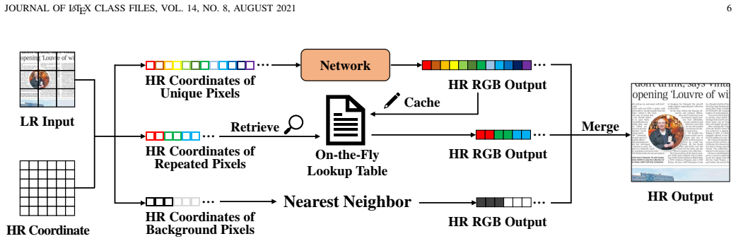
The two load-bearing mechanisms are (1) soft pixel binning with content attention in training and (2) the on-the-fly lookup table plus nearest-neighbor in inference. Soft binning assigns each pixel soft weights across N=10 uniformly spaced bins via a temperature-scaled exponential of distance to bin centers, preserving gradient flow; bins are merged into two content groups, and group-mean features are pooled spatially and broadcast back, yielding a content-dependent, non-local receptive field for every pixel. In inference, HR pixels are keyed by the RGB values of the nearest 3x3 LR patch plus the relative HR coordinate; the on-the-fly lookup table caches outputs for unique pixels and serves
What would settle it
Measure, on the SCI1K test set, how often the on-the-fly lookup table returns a prediction that differs from running the full network on the same 'repeated' pixel inputs, and compute the resulting PSNR difference; if the mismatch rate is non-negligible or the PSNR gap exceeds the reported fluctuation bounds, the lookup-table equivalence claim fails. A simpler version: count the fraction of repeated pixels whose cached key collides with a unique pixel but whose encoder feature (before the decoder) is not identical.
Extended reading notes
Core claim
PixelSR's central discovery is that pixel-level classification, rather than window or sub-image classification, is the right granularity for efficient screen-content SR. During training, soft binning discretizes pixels into two content-dependent groups—sharp screen-content edges vs. the rest—and spatial average pooling of each group yields a content attention vector that is broadcast back to every pixel, effectively enlarging the receptive field beyond the local 3x3 patch used by the implicit neural representation decoder. During inference, the method exploits self-repetitiveness and flatness: targeted HR pixels whose nearest 3x3 LR patch has equal RGB values are background pixels handled by
Load-bearing premise
The speedup collapses if two pixels with the same 3x3 local patch and the same relative coordinate do not reliably get the same network output—which the paper assumes without measuring, while the encoder's global receptive field could in principle make distant context change the prediction.
Editorial extensions
If this is right
- PixelSR achieves state-of-the-art PSNR on SCI1K, SCID, and SIQAD at in-training scales (e.g., 33.52 dB vs 32.80 dB at x3 on SCI1K with EDSR backbone) and maintains the lead at out-of-training scales up to x10.
- Total inference time on the SCI1K test set is shorter than LIIF, ITSRN, LTE, and BTC at every tested scale factor, with no PSNR drop attributable to the lookup table.
- The on-the-fly lookup table is a plug-in accelerator: the paper shows it reduces inference time for LIIF, ITSRN, LTE, BTC, and PixelSR alike, with PSNR fluctuations within small values.
- The content attention from soft binning gives a content-dependent and unlimited receptive field, which is the mechanism behind the accuracy gains; ablation shows 10 bins and a single conv layer are the best settings.
- The method generalizes across backbones (EDSR-baseline and SwinIR-light) and to other screen-content benchmarks, indicating the classification scheme, not extra capacity, drives the gains (all models ~1.6-1.9M params).
Reading between the lines
- If the lookup-table key is truly sufficient, the same trick should transfer to other content with repetitive structure—e.g., UI screenshots, CAD drawings, or document scans—suggesting a testable extension: measure the speedup and PSNR on such corpora to see where the repetition statistics break down.
- A direct falsifier is suggested by the paper's own design: because the encoder backbone has a global receptive field through downsampling layers, two pixels with identical 3x3 local patches and relative offsets can still receive different encoder features; one could quantify mismatch frequency and show whether errors accumulate as scale increases.
- The repetition statistics (20.90% background, 42.25% repeated patches in SCI1K vs 2.08% and 3.51% in DIV2K) imply the speedup is a property of the dataset, not the model; a natural next step is content-adaptive routing that decides per patch whether to run the network or the lookup table, making the method robust to mixed content.
Editorial analysis
A structured set of objections, weighed in public.
Referee Report
Summary. The paper proposes PixelSR, a screen-content super-resolution method with two components. In training, a lightweight content extractor plus soft pixel binning splits pixels into content-dependent groups; spatial average pooling within each group yields a content attention map that is concatenated to encoder features, giving every pixel a global, content-dependent receptive field. In inference, targeted HR pixels are classified as unique, repeated, or background. Unique pixels are processed by the network and their outputs cached in an on-the-fly lookup table keyed by the 3×3 LR patch RGB values and the relative HR coordinate; repeated pixels retrieve cached outputs; background pixels are generated by an unspecified nearest-neighbor scheme. Experiments on SCI1K, SCID, and SIQAD with EDSR and SwinIR-light backbones claim state-of-the-art PSNR at scales ×2–×10 and shorter total inference time on SCI1K without performance loss.
Significance. If the claims hold, PixelSR would be a meaningful contribution: it directly exploits two distinctive properties of screen content (uniform backgrounds and self-repetition) for both accuracy and speed, and it generalizes the caching idea to scale-arbitrary SR. The empirical breadth is a strength: three datasets, two backbone families, scales up to ×10, and comparisons to four strong baselines. The statistical evidence that background and repeated 3×3 patches are far more frequent in SCI1K than in DIV2K is a useful motivation. However, the central 'no performance loss' claim for the lookup table is not rigorously established, and one reported result contradicts the text. The paper currently does not ship code or machine-checked proofs, so the reproduction of the speedup and PSNR comparisons depends on the completeness of the experimental description.
major comments (4)
- [Sec. III-B, Table III] The central claim of 'faster inference without performance loss' rests on the on-the-fly lookup table's assumption that two pixels with the same (3×3 LR patch, relative coordinate) key receive identical network outputs. This is not guaranteed by the architecture: the EDSR/SwinIR encoders have receptive fields larger than 3×3, and F_CA in Eq. (6) is computed from whole-image group pooling (Eqs. 4–5), so the decoder input F_cat depends on distant context. Two pixels sharing the same local key can therefore produce different outputs. Table III only reports aggregate PSNR differences of 0.01–0.03 dB, with no per-pixel mismatch statistics, error bars, or significance test. Please add a direct measurement: run the full network for all pixels, compare predictions for repeated pixels against unique pixels with identical keys, and report the mismatch rate and its PSNR contribution. Alternatively,
- [Sec. IV-B, Table I] The text states that 'PixelSR consistently achieves the highest PSNR across all test sets at all scale factors' and 'ranks first across all scales' on SIQAD. Table I shows that on SIQAD at ×2, LTE achieves 33.29 dB while PixelSR achieves 33.25 dB. This contradicts the stated claim and affects the 'state-of-the-art' assertion. Please correct the claim or the table, and re-check every 'best' marker and the corresponding narrative.
- [Sec. IV-A / Sec. III-C] Reproducibility is hindered by missing settings and algorithmic details. The soft-binning temperature τ in Eq. (3) is never given a value, despite being a free parameter that controls the hardness of binning. The background nearest-neighbor algorithm is described only as 'use the nearest neighbor algorithm to generate HR pixels' without specifying the neighbor source, distance metric, or how it is applied at HR. These details are needed to reproduce the reported speed and quality numbers.
- [Table III vs. Table I] There is a numerical inconsistency: ITSRN without the lookup table at ×5 is reported as 26.52 dB in Table III but 26.72 dB in Table I. The inference-time methodology is also under-specified: what GPU, batch size, number of runs, and whether the timing includes the backbone encoder? The statement that 'inference time fluctuates within 1 second' is insufficient to assess the reported speedups.
minor comments (5)
- [Sec. IV-B] The text reports 'PixelSR achieves 28.54 dB on SCID at ×3 scale' with the SwinIR backbone, but Table II lists 28.59 dB; please harmonize.
- [Sec. III-B, Fig. 3] The statistical comparison of background and repeated patches should specify whether 3×3 patches are extracted with stride 1 or non-overlapping. The percentages differ substantially depending on this choice.
- [Sec. III-B] The statement that the on-the-fly lookup table is 'the first lookup table that can be used for scale arbitrary SR' is not substantiated by a comparison to prior arbitrary-scale LUT work; please soften or provide supporting references.
- [References] Some references are duplicated (e.g., [10]/[17], [5]/[18]) and some venue names are inconsistent (e.g., 'NeurIPS' vs. full conference name). Please clean the bibliography.
- [Abstract / Contributions] The phrase 'without the loss of model performance' should be qualified as 'with negligible PSNR difference on aggregate' unless per-pixel equivalence is proven; the current wording overstates the evidence.
Circularity Check
No significant circularity: the core PSNR and speed claims rest on a new architecture evaluated against external baselines; the lookup-table equivalence issue is a correctness/validity concern, not a circular reduction.
full rationale
The paper's derivation chain is self-contained. The content-attention module is a new feedforward computation defined by Eqs. 1-6, trained with L1 loss, and compared against external published methods (LIIF, ITSRN, LTE, BTC) on public screen-content benchmarks. No load-bearing step reduces to a fitted parameter renamed as a prediction. The number of bins, temperature, and group split are hyperparameters selected via ablations on the test set (Tables IV/V), which is a methodological weakness (test-set selection) but not a definitional circularity. The inference lookup table is an approximate caching scheme: the paper reports PSNR with and without the table (Table III) and finds small differences (0.00-0.03 dB). The claim that the 3x3 LR patch plus relative offset is a sufficient key is not guaranteed by the network's global receptive field, and no per-pixel mismatch statistics are provided; this is an unsupported equivalence and a validity risk, not a circular step, because the table output is not used to define the network output. The paper itself notes in V. Conclusion that the on-the-fly lookup table 'would not function well in natural images,' a scope limitation rather than a circularity. Self-citations in the references (e.g., [8], [9], [62]) are contextual and not load-bearing. Therefore, no significant circularity is identified.
Assumptions & free parameters
free parameters (4)
- bin temperature tau =
not reported
- number of bins N =
10
- group split P =
P=1 (first bin vs rest)
- content extractor layer count/kernel =
1 layer, 3x3 kernel
assumptions (3)
- domain assumption Exact equality of 3x3 RGB patch + relative distance implies (nearly) identical network output for the target pixel
- domain assumption Background pixels (flat 3x3 LR patch) are best upscaled by nearest-neighbor, i.e., their HR neighborhood is also flat
- domain assumption Screen-content datasets are representative of the deployment distribution and bicubic downsampling is the right degradation model
Cite this review
Pith. "Pith review of PixelSR: Efficient Screen Content Super-Resolution via Pixel Classification." pith.science (2026). https://pith.science/paper/2D4LRUBP
@misc{pith2026260800646,
  author       = {Pith},
  title        = {Pith review of: PixelSR: Efficient Screen Content Super-Resolution via Pixel Classification},
  year         = {2026},
  howpublished = {\url{https://pith.science/paper/2D4LRUBP}},
  note         = {Machine review of arXiv:2608.00646}
}
read the original abstract
Screen content images are generally composed of texts and graphics. Compared to natural images, these man-made images contain a large quantity of sharp but repetitive structures. However, existing works in screen content super-resolution underutilize the special characteristics of screen content, leaving a large room to improve model performance and speed up. In this paper, we propose PixelSR, a simple yet effective method to improve super-resolution performance but with faster inference speed. To improve model performance, we classify pixels via pixel binning to compute content attention in the training phase. Specifically, after binning pixels into content-dependent groups, content attention is aggregated from pixel features within each group to introduce a content-dependent and non-local receptive field for every pixel. In the testing phase, we utilize the properties of self-repetitiveness and redundancy in screen content to speed up inference without the loss of model performance. We divide targeted high-resolution pixels into three types, which are unique pixels, repeated pixels, and background pixels for each test image. We conduct conventional network processing on unique pixels and cache their predictions in the on-the-fly lookup table. For repeated pixels which have appeared in unique pixels, we directly retrieve prediction results from the lookup table without network processing. For background pixels, we use the nearest neighbor algorithm to generate high-resolution pixels. The on-the-fly lookup table is cleaned and repeats the procedure above for the next test image. Experiments show our PixelSR achieves state-of-the-art performance with shorter inference time in screen content super-resolution.
Figures


Figures from the paper (7 more)


Reference graph
Works this paper leans on
-
[30]
Accelerating image super- resolution networks with pixel-level classification,
J. Jeong, J. Kim, Y . Jo, and S. J. Kim, “Accelerating image super- resolution networks with pixel-level classification,”arXiv preprint arXiv:2407.21448, 2024. 1, 3
arXiv 2024
-
[1]
Deep learning for single image super-resolution: A brief review,
W. Yang, X. Zhang, Y . Tian, W. Wang, J.-H. Xue, and Q. Liao, “Deep learning for single image super-resolution: A brief review,”TMM, vol. 21, no. 12, pp. 3106–3121, 2019. 1
2019
-
[2]
Single-image super-resolution: A benchmark,
C.-Y . Yang, C. Ma, and M.-H. Yang, “Single-image super-resolution: A benchmark,” inECCV, 2014, pp. 372–386. 1
2014
-
[3]
Transformer for single image super-resolution,
Z. Lu, J. Li, H. Liu, C. Huang, L. Zhang, and T. Zeng, “Transformer for single image super-resolution,” inCVPR, 2022, pp. 457–466. 1
2022
-
[4]
Single image super-resolution from transformed self-exemplars,
J.-B. Huang, A. Singh, and N. Ahuja, “Single image super-resolution from transformed self-exemplars,” inCVPR, 2015, pp. 5197–5206. 1
2015
-
[6]
Single-image super-resolution using sparse regression and natural image prior,
K. I. Kim and Y . Kwon, “Single-image super-resolution using sparse regression and natural image prior,”TPAMI, vol. 32, no. 6, pp. 1127– 1133, 2010. 1
2010
-
[7]
Second-order attention network for single image super-resolution,
T. Dai, J. Cai, Y . Zhang, S.-T. Xia, and L. Zhang, “Second-order attention network for single image super-resolution,” inCVPR, 2019, pp. 11 065–11 074. 1
2019
-
[8]
Structure-preserving image super- resolution,
C. Ma, Y . Rao, J. Lu, and J. Zhou, “Structure-preserving image super- resolution,”TPAMI, vol. 44, no. 11, pp. 7898–7911, 2021. 1
2021
Show all 69 references
-
[9]
Structure- preserving super resolution with gradient guidance,
C. Ma, Y . Rao, Y . Cheng, C. Chen, J. Lu, and J. Zhou, “Structure- preserving super resolution with gradient guidance,” inCVPR, 2020, pp. 7769–7778. 1
2020
-
[10]
Limits on super-resolution and how to break them,
S. Baker and T. Kanade, “Limits on super-resolution and how to break them,”TPAMI, vol. 24, no. 9, pp. 1167–1183, 2002. 1
2002
-
[11]
Deep networks for image super-resolution with sparse prior,
Z. Wang, D. Liu, J. Yang, W. Han, and T. Huang, “Deep networks for image super-resolution with sparse prior,” inICCV, 2015, pp. 370–378. 1
2015
-
[12]
Multi-scale residual network for image super-resolution,
J. Li, F. Fang, K. Mei, and G. Zhang, “Multi-scale residual network for image super-resolution,” inECCV, 2018, pp. 517–532. 1
2018
-
[13]
Deep burst super- resolution,
G. Bhat, M. Danelljan, L. Van Gool, and R. Timofte, “Deep burst super- resolution,” inCVPR, 2021, pp. 9209–9218. 1
2021
-
[14]
Deep learning for image super- resolution: A survey,
Z. Wang, J. Chen, and S. C. Hoi, “Deep learning for image super- resolution: A survey,”TPAMI, vol. 43, pp. 3365–3387, 2020. 1
2020
-
[15]
A survey on super-resolution imaging,
J. Tian and K.-K. Ma, “A survey on super-resolution imaging,”SIGNAL IMAGE VIDEO P, vol. 5, pp. 329–342, 2011. 1 JOURNAL OF LATEX CLASS FILES, VOL. 14, NO. 8, AUGUST 2021 13
2011
-
[16]
Anycost network quantization for image super-resolution,
J. Zhang, Z. Wang, H. Wang, J. Zhou, and J. Lu, “Anycost network quantization for image super-resolution,”TIP, vol. 33, pp. 2279–2292,
-
[17]
Limits on super-resolution and how to break them,
S. Baker and T. Kanade, “Limits on super-resolution and how to break them,”IEEE transactions on pattern analysis and machine intelligence, vol. 24, pp. 1167–1183, 2002. 1
2002
-
[18]
Super-resolution from a single image,
D. Glasner, S. Bagon, and M. Irani, “Super-resolution from a single image,” inICCV, 2009, pp. 349–356. 1
2009
-
[19]
Space-time super-resolution,
E. Shechtman, Y . Caspi, and M. Irani, “Space-time super-resolution,” TPAMI, vol. 27, pp. 531–545, 2005. 1
2005
-
[20]
Learning a deep convolutional network for image super-resolution,
C. Dong, C. C. Loy, K. He, and X. Tang, “Learning a deep convolutional network for image super-resolution,” inECCV, 2014, pp. 184–199. 1
2014
-
[21]
Image super-resolution using deep convolutional networks,
——, “Image super-resolution using deep convolutional networks,” TPAMI, vol. 38, pp. 295–307, 2015. 1
2015
-
[22]
Statistical performance analysis of super- resolution,
D. Robinson and P. Milanfar, “Statistical performance analysis of super- resolution,”IEEE Transactions on Image Processing, vol. 15, pp. 1413– 1428, 2006. 1
2006
-
[23]
Bayesian image super-resolution,
M. Tipping and C. Bishop, “Bayesian image super-resolution,”NeurIPS, vol. 15, 2002. 1
2002
-
[24]
Learning texture transformer network for image super-resolution,
F. Yang, H. Yang, J. Fu, H. Lu, and B. Guo, “Learning texture transformer network for image super-resolution,” inCVPR, 2020, pp. 5791–5800. 1
2020
-
[25]
Masa-sr: Matching acceleration and spatial adaptation for reference-based image super-resolution,
L. Lu, W. Li, X. Tao, J. Lu, and J. Jia, “Masa-sr: Matching acceleration and spatial adaptation for reference-based image super-resolution,” in CVPR, 2021, pp. 6368–6377. 1
2021
-
[26]
B-spline texture coefficients estimator for screen content image super-resolution,
B. Pak, J. Lee, and K. H. Jin, “B-spline texture coefficients estimator for screen content image super-resolution,” inCVPR, 2023, pp. 10 062– 10 071. 1, 2, 3, 6, 7, 8, 9, 10, 12
2023
-
[27]
Perceptual quality assessment of screen content images,
H. Yang, Y . Fang, and W. Lin, “Perceptual quality assessment of screen content images,”TIP, no. 11, pp. 4408–4421, 2015. 1, 3, 6
2015
-
[28]
Classsr: A general framework to accelerate super-resolution networks by data characteristic,
X. Kong, H. Zhao, Y . Qiao, and C. Dong, “Classsr: A general framework to accelerate super-resolution networks by data characteristic,” inCVPR, 2021, pp. 12 016–12 025. 1, 3
2021
-
[29]
Camixersr: Only details need more
Y . Wang, S. Zhao, Y . Liu, J. Li, and L. Zhang, “Camixersr: Only details need more" attention",”arXiv preprint arXiv:2402.19289, 2024. 1, 3
2024 arXiv
-
[31]
Ciaosr: Continuous implicit attention-in- attention network for arbitrary-scale image super-resolution,
J. Cao, Q. Wang, Y . Xian, Y . Li, B. Ni, Z. Pi, K. Zhang, Y . Zhang, R. Timofte, and L. Van Gool, “Ciaosr: Continuous implicit attention-in- attention network for arbitrary-scale image super-resolution,” inCVPR, 2023, pp. 1796–1807. 1, 2, 3
2023
-
[32]
Image super-resolution with cross-scale non-local attention and exhaustive self- exemplars mining,
Y . Mei, Y . Fan, Y . Zhou, L. Huang, T. S. Huang, and H. Shi, “Image super-resolution with cross-scale non-local attention and exhaustive self- exemplars mining,” inCVPR, 2020, pp. 5690–5699. 1, 3
2020
-
[33]
Image processing gnn: Breaking rigidity in super-resolution,
Y . Tian, H. Chen, C. Xu, and Y . Wang, “Image processing gnn: Breaking rigidity in super-resolution,” inCVPR, 2024, pp. 24 108–24 117. 1, 3
2024
-
[34]
Learning continuous image representa- tion with local implicit image function,
Y . Chen, S. Liu, and X. Wang, “Learning continuous image representa- tion with local implicit image function,” inCVPR, 2021, pp. 8628–8638. 2, 3, 6, 7, 8, 9, 10, 12
2021
-
[35]
Implicit transformer network for screen content image continuous super-resolution,
J. Yang, S. Shen, H. Yue, and K. Li, “Implicit transformer network for screen content image continuous super-resolution,”NeurIPS, pp. 13 304– 13 315, 2021. 2, 3, 5, 6, 7, 8, 9, 10, 12
2021
-
[36]
Local texture estimator for implicit representation function,
J. Lee and K. H. Jin, “Local texture estimator for implicit representation function,” inCVPR, 2022, pp. 1929–1938. 2, 3, 7, 8, 9, 10, 12
2022
-
[38]
Learning a single network for scale-arbitrary super-resolution,
L. Wang, Y . Wang, Z. Lin, J. Yang, W. An, and Y . Guo, “Learning a single network for scale-arbitrary super-resolution,” inICCV, 2021, pp. 4801–4810. 2
2021
-
[39]
Deep arbitrary- scale image super-resolution via scale-equivariance pursuit,
X. Wang, X. Chen, B. Ni, H. Wang, Z. Tong, and Y . Liu, “Deep arbitrary- scale image super-resolution via scale-equivariance pursuit,” inCVPR, 2023, pp. 1786–1795. 2
2023
-
[40]
Ultrasr: Spatial encoding is a missing key for implicit image function-based arbitrary-scale super-resolution,
X. Xu, Z. Wang, and H. Shi, “Ultrasr: Spatial encoding is a missing key for implicit image function-based arbitrary-scale super-resolution,” arXiv preprint arXiv:2103.12716, 2021. 2
2021 arXiv
-
[41]
Local implicit normalizing flow for arbitrary-scale image super- resolution,
J.-E. Yao, L.-Y . Tsao, Y .-C. Lo, R. Tseng, C.-C. Chang, and C.-Y . Lee, “Local implicit normalizing flow for arbitrary-scale image super- resolution,” inCVPR, 2023, pp. 1776–1785. 2
2023
-
[42]
Cascaded local implicit transformer for arbitrary-scale super- resolution,
H.-W. Chen, Y .-S. Xu, M.-F. Hong, Y .-M. Tsai, H.-K. Kuo, and C.- Y . Lee, “Cascaded local implicit transformer for arbitrary-scale super- resolution,” inCVPR, 2023, pp. 18 257–18 267. 2
2023
-
[43]
Activating more information in arbitrary-scale image super-resolution,
Y . Zhao, Q. Teng, H. Chen, S. Zhang, X. He, Y . Li, and R. E. Sheriff, “Activating more information in arbitrary-scale image super-resolution,” TMM, vol. 26, pp. 7946–7961, 2024. 2
2024
-
[44]
Recovering realistic details for magnification-arbitrary image super-resolution,
C. Ma, P. Yu, J. Lu, and J. Zhou, “Recovering realistic details for magnification-arbitrary image super-resolution,”TIP, vol. 31, pp. 3669– 3683, 2022. 2
2022
-
[45]
Hiif: Hierarchical encoding based implicit image function for continuous super-resolution,
Y . Jiang, H. M. Kwan, T. Peng, G. Gao, F. Zhang, X. Zhu, J. Sole, and D. Bull, “Hiif: Hierarchical encoding based implicit image function for continuous super-resolution,” inCVPR, 2025, pp. 2289–2299. 2
2025
-
[46]
Meta-sr: A magnification-arbitrary network for super-resolution,
X. Hu, H. Mu, X. Zhang, Z. Wang, T. Tan, and J. Sun, “Meta-sr: A magnification-arbitrary network for super-resolution,” inCVPR, 2019, pp. 1575–1584. 2
2019
-
[47]
Learning based screen image compres- sion,
H. Yang, W. Lin, and C. Deng, “Learning based screen image compres- sion,” inMMSPW, 2012, pp. 77–82. 3
2012
-
[48]
Super resolution for compressed screen content video,
M. Wang, J. Xu, L. Zhang, J. Li, and S. Wang, “Super resolution for compressed screen content video,” inDCC, 2021, pp. 173–182. 3
2021
-
[49]
Itsrn++: Stronger and better implicit transformer network for continuous screen content image super- resolution,
S. Shen, H. Yue, J. Yang, and K. Li, “Itsrn++: Stronger and better implicit transformer network for continuous screen content image super- resolution,”arXiv, 2022. 3
2022
-
[50]
Real-time single image and video super- resolution using an efficient sub-pixel convolutional neural network,
W. Shi, J. Caballero, F. Huszár, J. Totz, A. P. Aitken, R. Bishop, D. Rueckert, and Z. Wang, “Real-time single image and video super- resolution using an efficient sub-pixel convolutional neural network,” in CVPR, 2016, pp. 1874–1883. 3
2016
-
[51]
Fast, accurate, and lightweight super-resolution with cascading residual network,
N. Ahn, B. Kang, and K.-A. Sohn, “Fast, accurate, and lightweight super-resolution with cascading residual network,” inECCV, 2018, pp. 252–268. 3
2018
-
[52]
Lightweight image super- resolution with information multi-distillation network,
Z. Hui, X. Gao, Y . Yang, and X. Wang, “Lightweight image super- resolution with information multi-distillation network,” inACM MM, 2019, pp. 2024–2032. 3
2019
-
[53]
Enhanced deep residual networks for single image super-resolution,
B. Lim, S. Son, H. Kim, S. Nah, and K. Mu Lee, “Enhanced deep residual networks for single image super-resolution,” inCVPRW, 2017, pp. 136–144. 3, 6, 7
2017
-
[54]
Lattice network for lightweight image restoration,
X. Luo, Y . Qu, Y . Xie, Y . Zhang, C. Li, and Y . Fu, “Lattice network for lightweight image restoration,”TPAMI, no. 4, pp. 4826–4842, 2022. 3
2022
-
[55]
Dlgsanet: lightweight dynamic local and global self-attention networks for image super-resolution,
X. Li, J. Dong, J. Tang, and J. Pan, “Dlgsanet: lightweight dynamic local and global self-attention networks for image super-resolution,” in ICCV, 2023, pp. 12 792–12 801. 3
2023
-
[56]
Accelerating the super-resolution convolutional neural network,
C. Dong, C. C. Loy, and X. Tang, “Accelerating the super-resolution convolutional neural network,” inECCV, 2016, pp. 391–407. 3
2016
-
[57]
Ntire 2023 challenge on efficient super- resolution: Methods and results,
Y . Li, Y . Zhang, R. Timofte, L. Van Gool, L. Yu, Y . Li, X. Li, T. Jiang, Q. Wu, M. Hanet al., “Ntire 2023 challenge on efficient super- resolution: Methods and results,” inCVPR, 2023, pp. 1921–1959. 3
2023
-
[58]
Global aligned structured sparsity learning for efficient image super-resolution,
H. Wang, Y . Zhang, C. Qin, L. Van Gool, and Y . Fu, “Global aligned structured sparsity learning for efficient image super-resolution,”TPAMI,
-
[59]
Lmlt: Low-to-high multi-level vision transformer for lightweight image super-resolution,
J. Kim, J. Nang, and J. Choe, “Lmlt: Low-to-high multi-level vision transformer for lightweight image super-resolution,” inICCV, 2025, pp. 5509–5519. 3
2025
-
[60]
Practical single-image super-resolution using look- up table,
Y . Jo and S. J. Kim, “Practical single-image super-resolution using look- up table,” inCVPR, 2021, pp. 691–700. 3
2021
-
[61]
Mulut: Cooperating multiple look-up tables for efficient image super-resolution,
J. Li, C. Chen, Z. Cheng, and Z. Xiong, “Mulut: Cooperating multiple look-up tables for efficient image super-resolution,” inECCV, 2022, pp. 238–256. 3
2022
-
[62]
Learning series-parallel lookup tables for efficient image super-resolution,
C. Ma, J. Zhang, J. Zhou, and J. Lu, “Learning series-parallel lookup tables for efficient image super-resolution,” inECCV, 2022, pp. 305–
2022
-
[63]
Reconstructed convolution module based look-up tables for efficient image super- resolution,
G. Liu, Y . Ding, M. Li, M. Sun, X. Wen, and B. Wang, “Reconstructed convolution module based look-up tables for efficient image super- resolution,” inICCV, 2023, pp. 12 217–12 226. 3
2023
-
[64]
Arm: Any-time super-resolution method,
B. Chen, M. Lin, K. Sheng, M. Zhang, P. Chen, K. Li, L. Cao, and R. Ji, “Arm: Any-time super-resolution method,” inECCV, 2022, pp. 254–270. 3
2022
-
[65]
Cabm: Content- aware bit mapping for single image super-resolution network with large input,
S. Tian, M. Lu, J. Liu, Y . Guo, Y . Chen, and S. Zhang, “Cabm: Content- aware bit mapping for single image super-resolution network with large input,” inCVPR, 2023, pp. 1756–1765. 3
2023
-
[66]
Autolut: Lut-based image super-resolution with automatic sampling and adaptive residual learning,
Y . Xu, S. Yang, X. Liu, J. Liu, J. Tang, and G. Wu, “Autolut: Lut-based image super-resolution with automatic sampling and adaptive residual learning,” inCVPR, 2025, pp. 23 131–23 140. 3
2025
-
[67]
Ntire 2017 challenge on single image super-resolution: Dataset and study,
E. Agustsson and R. Timofte, “Ntire 2017 challenge on single image super-resolution: Dataset and study,” inCVPRW, 2017, pp. 126–135. 5
2017
-
[68]
Esim: Edge similarity for screen content image quality assessment,
Z. Ni, L. Ma, H. Zeng, J. Chen, C. Cai, and K.-K. Ma, “Esim: Edge similarity for screen content image quality assessment,”TIP, no. 10, pp. 4818–4831, 2017. 6
2017
-
[69]
Swinir: Image restoration using swin transformer,
J. Liang, J. Cao, G. Sun, K. Zhang, L. Van Gool, and R. Timofte, “Swinir: Image restoration using swin transformer,” inICCV, 2021, pp. 1833–1844. 6, 7
2021
-
[70]
Adam: A method for stochastic optimization,
D. P. Kingma and J. Ba, “Adam: A method for stochastic optimization,” arXiv, 2014. 6
2014
-
[71]
Scene text recognition with permuted autoregressive sequence models,
D. Bautista and R. Atienza, “Scene text recognition with permuted autoregressive sequence models,” inECCV, 2022, pp. 178–196. 8
2022
Reviewed August 4, 2026 · model on record in the stance chip above.
Discussion (0). Sign in to comment.