REVIEW 3 major objections 4 minor 35 references
Simulation-free and finite-time diffusion model
T0 review · 3 major / 4 minor · reviewed 2026-08-15 · deepseek-v4-flash
Pith's one-line read Prescribing time-dependent conditional distributions yields a diffusion reference process that trains without simulation and connects prior to data at a fixed finite horizon.
desk verdict A clean unifying framework for reference processes, but the finite-time claim is undercut by a singular objective that the paper only truncates, and novelty is modest given Stochastic Interpolants. read the letter →
The pith
A machine-rendered reading of the paper's core claim, the machinery that carries it, and where it could break.
The reading
What carries the argument
The central machinery is the inversion of the design order: instead of specifying a reference SDE and deriving its marginals, the paper prescribes conditional distributions $\{\rho_t(\cdot|x)\}$ and solves for the SDE coefficients via the conditional Fokker–Planck equation (19), $\partial_t \rho_t = -\nabla_z\cdot(\alpha\rho_t) + \tfrac12 \nabla_z\cdot(\nabla_z(\Gamma\rho_t))$, with $\Gamma=bb^\top$. The reference drift at a point is the conditional-drift average $a(t,z)=\int \alpha(t,z,x)\rho_t(z|x)\mu(x)/p_t(z)\,dx$, and substituting this into the Girsanov objective yields (23), whose minimizer matches the full KL objective. The practical Gaussian instance chooses $\rho_t(z|x)=\mathcal{N}(z;tx,(1-t)^2 I_d)$ with $\lambda(t)=\sigma(t)^{-1}$, giving the explicit simulation-free objective (48); the non-Gaussian instance uses a push-forward family $\phi^x_t(y)=f_t(y+g_t(x))$, which guarantees an $x$-independent diffusion coefficient so that the same objective applies.
What would settle it
Train the Gaussian-prior model on truncation horizons $[0,1-\delta]$ with $\delta = 10^{-2}, 10^{-3}, 10^{-4}$ and measure sample quality (e.g., MMD) as a function of $\delta$; if quality degrades monotonically as $\delta\to 0$ or the loss diverges, the truncation is load-bearing and the objective is ill-posed without it. Alternatively, numerically integrate (48) with the trained network to check whether the expected loss over $t\in[0,1)$ is finite.
Extended reading notes
Core claim
The paper claims that the reference process in a diffusion model can be constructed by first prescribing a family of tractable conditional distributions $\{\rho_t(\cdot|x)\}_{t\in[0,1]}$ with the boundary conditions $p_0=\pi$ and $p_1=\mu$ for the marginals $p_t(z)=\int \rho_t(z|x)\mu(x)\,dx$, and then computing SDE coefficients $(\alpha,b)$ that solve the conditional Fokker–Planck equation (19). The resulting reference SDE $dZ_t=a(t,Z_t)dt+b(t,Z_t)dW_t$ has marginals $p_t$, and the path-space KL objective $\mathcal{L}_{\mathrm{DM}}$ is, up to a $\theta$-independent constant, equal to the simulation-free objective $\mathcal{L}_{\mathrm{SF}}$ in (23), which requires only direct sampling from $\rho_t$ and evaluation of the conditional drift $\alpha$. This removes the need to simulate the reference SDE during training and, because the marginals connect $\pi$ to $\mu$ over $[0,1]$, gives finite-time generation. The paper further claims that score matching is an artifact of reversing a data-to-prior process: the score $\nabla\log p_t$ never enters $\mathcal{L}_{\mathrm{SF}}$, and conditional flow matching is recovered as the small-noise limit ($\epsilon\to 0$) of the stochastic construction.
Load-bearing premise
The practical schedules make the training objective singular at the terminal time $t=1$, and the paper trains on $[0,0.99]$ while treating the endpoint as a limit; if that limit is not well-defined, the claimed finite-time connection holds only as a truncated approximation.
Editorial extensions
If this is right
- A diffusion model can be trained with the objective in (23) (explicitly (48) for the Gaussian schedule) using only reparameterized samples from the prescribed conditionals, never simulating the reference SDE, and the generation process still connects prior to data at the fixed time $t=1$.
- Score matching is not a necessary component of diffusion-model training: the score $\nabla\log p_t$ does not appear in the new objective, and it only enters conventional models because their reference process is defined in the data-to-prior direction and then time-reversed.
- Conditional flow matching is recovered as the small-noise limit $\epsilon\to 0$ of the stochastic construction, giving CFM a path-space KL interpretation that it lacks on its own.
- The framework extends to non-Gaussian priors by using a push-forward bijection family of the form $\phi^x_t(y)=f_t(y+g_t(x))$, so heavy-tailed priors can be used without sacrificing simulation-free training.
Reading between the lines
- The explicit $1/(1-t)$ weight in the practical objectives (48) and (52) implies that for any fixed network with bounded output, the untruncated expected loss over $t\in[0,1)$ is infinite; if so, the finite-time claim requires a proof that the $\tau\to1$ limit is finite and a statement of the truncation bias at $t=0.99$.
- The construction suggests that diffusion models, conditional flow matching, and stochastic interpolants can be viewed as different choices of the same design object — the conditional path $\{\rho_t(\cdot|x)\}$ and a noise level — which may simplify comparing and transferring hyperparameters between methods.
- Since the interpolation schedule affects generation quality even with fixed boundary distributions, learning the schedule $\varphi(t)$ as part of the objective appears to be a natural and testable extension, and the paper's metric tables provide a benchmark that such learned schedules would need to beat.
Signed reviews
Editorial analysis
A structured set of objections, weighed in public.
Referee Report
Summary. The paper proposes a framework for designing the reference diffusion process in generative diffusion models by first prescribing tractable conditional distributions rho_t(z|x) and then constructing an SDE whose marginals realize them. With boundary conditions p_0=pi and p_1=mu, the construction is claimed to achieve simulation-free training and finite-time generation simultaneously. The resulting objective L_SF in Eq. (23) is shown, up to a theta-independent constant, to be equivalent to a path-space KL divergence, and the paper argues that score matching is not fundamental but emerges from time reversal, while conditional flow matching is recovered as a small-noise limit. Experiments on four two-dimensional toy datasets with Gaussian and Johnson's SU priors illustrate the method.
Significance. If the claims are established, the paper makes a useful conceptual contribution: it offers a constructive way to break the usual trade-off between simulation-free training and finite-time generation, and it provides a unified viewpoint connecting score matching, conditional flow matching, and stochastic localization. The algebraic derivations in Sec. III and Appendices A-D are internally consistent, and the small-noise limit leading to Eq. (39) is a clean observation. The paper also ships open-source code and checkpoints and includes a fair, if small-scale, comparison with a VP-SBM. However, the concrete schedules used in the experiments make the proposed objective ill-defined on the full time interval, and the advertised finite-time equivalence is asserted through an unanalyzed limit; these issues currently prevent the central claim from being accepted as proven.
major comments (3)
- [Sec. VI.A, Eq. (48); Sec. III, Eq. (23)] With m_t(x)=tx, sigma(t)=1-t, and lambda(t)=sigma(t)^{-1}, the objective Eq. (23) is not finite on the full interval [0,1]. For the perfectly representable network s_theta=0, Eq. (48) evaluates to (1/(2n)) sum_i integral_0^1 dt (E_xi ||x_i - (3/2)xi||^2)/(1-t) = infinity whenever the data have finite second moment. Thus the zero network alone makes the purported objective infinite, and the theta-independent constant discarded in Appendix A also diverges. The statement in Sec. VI.A that 't=1 is not sampled' is a truncation, not a justification: no bound on the omitted tail [0.99,1] or on the resulting bias is supplied. This directly undermines the claim that Eq. (23) is a tractable simulation-free objective equivalent to the path-space KL in Eq. (22) on the full interval.
- [Sec. IV, first paragraph] The paper defines the Girsanov representation Eq. (22) by applying it on [0,tau] with tau<1 and then taking the limit tau->1, because the chosen diffusion coefficient degenerates at t=1. No theorem is given that this limit is well-defined, finite, or that it preserves the terminal-marginal constraint p_1=mu in a sense compatible with the objective. Since b(1)=0 and the drift alpha contains terms of order (1-t)^{-1}, the standard hypotheses of the Girsanov theorem are not verified on [0,1]. Consequently the advertised 'finite-time' connection and the equivalence to Eq. (22) are presently asserted only in a limiting sense; the paper needs either a proof for the chosen schedules or a non-degenerate schedule for which the objective is genuinely finite on [0,1].
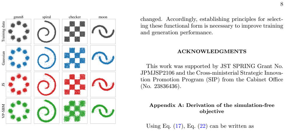
- [Sec. VI.B, Eq. (52); Sec. VI.C] The non-Gaussian-prior objective in Eq. (52) carries the same singular weight 1/(1-t) and is subject to the same truncation. The experiments in Fig. 1 therefore train and evaluate a truncated surrogate of Eq. (23), not the stated objective, and no analysis of truncation bias or of the influence of the singular endpoint is given. The main experimental section also reports only qualitative samples; quantitative metrics appear only for schedule comparisons in Appendix E.2. As a result, the numerical demonstration does not currently resolve the central theoretical concern about finiteness of the objective.
minor comments (4)
- [Eq. (28)] The notation for b(t) is ambiguous: it should be typeset explicitly as sqrt(lambda(t)) sigma(t) I_d (with parentheses), since Appendix B defines lambda via c(t)^2/sigma(t)^2 and the surrounding text can be misread as sqrt(lambda(t) sigma(t)) I_d.
- [Eq. (48) and surrounding text] The use of U[0,1) together with an integral over [0,1] is confusing when the integrand is singular at the endpoint; the paper should specify the truncated interval [0,1-epsilon] or explicitly describe the limiting procedure used in the Monte Carlo estimate.
- [Fig. 1] Quantitative metrics for the main Gaussian-prior and Johnson-SU-prior experiments would strengthen the comparison with VP-SBM; currently only qualitative sample plots are given in the main text.
- [Sec. V.A] The statement that 'score matching is not fundamental' would benefit from qualification: the non-Gaussian construction still uses grad log pi in Eq. (34), and Sec. V.C shows that score-like terms reappear when a deterministic flow is stochastically lifted.
Circularity Check
No significant circularity: the derivation is a constructive, self-contained framework; boundary conditions are imposed design choices, not fitted predictions.
full rationale
The paper's central derivation is constructive rather than circular. It prescribes a family of conditional distributions {ρ_t} satisfying boundary conditions p0=π and p1=μ (Eq. 18), then solves the conditional Fokker-Planck equation for α and b (Eqs. 19-21) and derives the simulation-free objective L_SF in Eq. (23) from the path-space KL via algebraic manipulation in Appendix A. The equivalence of minimizers between L_DM and L_SF is proven explicitly in Eq. (A6), not assumed. The Gaussian and non-Gaussian constructions in Sections IV.A and IV.B are derived from the prescribed ρ_t by direct calculation (Appendices B and C), with free functions m_t, σ, λ, γ, and φ as design choices. The small-noise limit recovering conditional flow matching (Eqs. 37-40) is a direct limit of the derived drift, not an imported ansatz. The cited prior work of the authors, e.g., Ref. [13], is used only as an example of Schrödinger bridge methods and is not load-bearing for the main derivation. The manuscript's own acknowledgment that t=1 is not sampled and that the objective has a singular weight at t=1 (Sec. VI.A) raises a mathematical/truncation-validity concern, but it is not circularity: the paper does not fit a parameter to data and then rename the fit as a prediction. The boundary conditions are imposed by construction, and the schedule choices are explicitly shown in Appendix E.2 to affect quality, confirming they are free design inputs rather than outputs smuggled into the claim. No self-citation chain, uniqueness theorem, or definitional equivalence forces the central result.
Assumptions & free parameters
free parameters (4)
- λ(t) =
1/σ(t) in experiments
- m_t(x) and σ(t) schedules =
m_t=t x, σ(t)=1-t in main experiments; φ(t) variants in Appendix E
- γ(t) =
1/(1-t) in experiments
- schedule parameter c in φ(t) =
0.8, -1, -1.8, -2, 2 for s-curve, n-curve, nn-curve, concave, convex
assumptions (5)
- standard math Girsanov theorem and path-space KL divergence
- standard math Fokker-Planck equation and Itô formula
- domain assumption Existence and uniqueness of the constructed SDE (20) with marginal p_t
- domain assumption Stationary distribution of (29) is π
- domain assumption Functional form (36) for ϕ^x_t
Cite this review
Pith. "Pith review of Simulation-free and finite-time diffusion model." pith.science (2026). https://pith.science/paper/2V4GXZRP
@misc{pith2026260803117,
  author       = {Pith},
  title        = {Pith review of: Simulation-free and finite-time diffusion model},
  year         = {2026},
  howpublished = {\url{https://pith.science/paper/2V4GXZRP}},
  note         = {Machine review of arXiv:2608.03117}
}
read the original abstract
The performance of generative diffusion models is determined by the choice of the reference diffusion process connecting the empirical and prior distributions. Conventional approaches typically trade off simulation-free training against finite-time generation. We propose a framework for designing the reference process that achieves both simultaneously. The key idea is to prescribe tractable time-dependent conditional distributions and then construct the reference process realizing them as its marginals. This framework reveals that score matching is not fundamental to diffusion-model training but instead emerges naturally through reversal of the reference process. We further show that conditional flow matching arises as the small-noise limit of the proposed framework.
Figures


Reference graph
Works this paper leans on
-
[1]
Fix an arbitraryx 0∈R d and define a smooth bijectionf t(y) :=ϕ x0 t (y)
By the inverse function theorem, Dyϕx t (ϕx t )−1(z) = [Dz(ϕx t )−1(z)]−1.(C2) Hence, the condition above implies thatD z(ϕx t )−1(z) is independent ofx. Fix an arbitraryx 0∈R d and define a smooth bijectionf t(y) :=ϕ x0 t (y). Since the Jacobians of (ϕx t )−1 andf −1 t with respect tozare identical, their dif- ference is independent ofz. Thus, there exis...
-
[2]
(47) andλ(t) =σ(t) −1 into Eqs
Gaussian prior By substituting Eq. (47) andλ(t) =σ(t) −1 into Eqs. (27) and (28), we obtain α(t,z,x) =x+ − 1 1−t − 1 2 1 1−t (z−tx) =x− 3 2 z−tx 1−t , (D1) b(t,z) = √ 1−tI d.(D2) By employing the reparameterization trick in Eq. (26) into the above equation, we getαas a function ofξin- stead ofz: α(t,tx+ (1−t)ξ,x) =x− 3 2ξ.(D3) Therefore, the expectation v...
-
[3]
Johnson’sS U prior From the definition of the Johnson’sS U distribution Eq. (49), the gradient of its log-density is ∇y logπ(y) =− sinh−1yp 1 +y 2− y 1 +y 2.(D5) Substituting Eq. (51) andγ(t) = 1/(1−t) into Eqs. (34) and (35) gives α(t,tx+ (1−t)y,x) =x−y− 1 2 sinh−1yp 1 +y 2 + y 1 +y 2 ! . (D6) Also,b(t,z) = √1−tI d. Furthermore, the reparameteri- zation ...
-
[4]
Figure 2 shows generated samples for T= 1,10,100, where the number of discretization steps (i.e
Effect of the time horizon in VP-SBM We examined the sensitivity of the VP-SBM to the time horizonT. Figure 2 shows generated samples for T= 1,10,100, where the number of discretization steps (i.e. Euler–Maruyama steps) was fixed to 100 in all cases, as in the setting in Sec. VI. The results for differentTreveal a trade-off between training and generation...
-
[5]
Effect of the interpolation schedule We demonstrate that the performance depends on the design of the reference process realizing the prescribed 11 FIG. 2. The visualization of 7,500 training data and gen- erated samples from VP-SBMs. The top row represents the training data. The remaining rows show samples from the VP-SBM withT= 1,10,100, respectively. A...
-
[6]
We consider the linear scheduleφ(t) =tin Eq. (47) together with cubic and exponential families: φ(t) = (1−c)t+ 3ct 2−2ct 3, φ(t) = ect−1 ec−1 ,(E2) wherecis an arbitrary parameter. The values of the parametercare summarized in Table I, and the corre- sponding schedule curves are shown in Fig. 3. Substituting Eq. (E1) andλ(t) =σ(t) −1 into Eqs. (27) and (2...
-
[7]
J. Sohl-Dickstein, E. Weiss, N. Maheswaranathan, and S. Ganguli, Deep unsupervised learning using nonequi- librium thermodynamics, inInternational Conference on 12 FIG. 3. Interpolation schedulesφ(t) used in the additional experiments. All schedules satisfyφ(0) = 0 andφ(1) = 1, but differ in their intermediate time dependence. TABLE II. The mean of MMD ov...
-
[8]
J. Ho, A. Jain, and P. Abbeel, Denoising diffusion prob- abilistic models, inAdvances in Neural Information Pro- cessing Systems, Vol. 33 (Curran Associates, Inc., 2020) pp. 6840–6851
work page 2020
Show all 35 references
-
[9]
Y. Song, J. Sohl-Dickstein, D. P. Kingma, A. Kumar, S. Ermon, and B. Poole, Score-based generative modeling through stochastic differential equations (2021)
2021
-
[10]
Croitoru, V
F.-A. Croitoru, V. Hondru, R. T. Ionescu, and M. Shah, Diffusion models in vision: A survey, IEEE transactions on pattern analysis and machine intelligence45, 10850 TABLE III. The mean of SWD over 10 independent training runs with different random seeds for each dataset and cu...
2023
-
[11]
Zhang, C
C. Zhang, C. Zhang, S. Zheng, M. Zhang, M. Qamar, S.-H. Bae, and I. S. Kweon, A survey on audio diffusion models: Text to speech synthesis and enhancement in generative ai, arXiv preprint arXiv:2303.13336 (2023)
2023 arXiv
-
[12]
Z. Xing, Q. Feng, H. Chen, Q. Dai, H. Hu, H. Xu, Z. Wu, and Y.-G. Jiang, A survey on video diffusion models, ACM Computing Surveys57, 1 (2024)
2024
-
[13]
S. Nie, F. Zhu, Z. You, X. Zhang, J. Ou, J. Hu, J. Zhou, Y. Lin, J.-R. Wen, and C. Li, Large language diffusion models, Advances in Neural Information Processing Sys- tems38, 50608 (2026)
2026
-
[14]
Y. Song, C. Durkan, I. Murray, and S. Ermon, Maxi- mum likelihood training of score-based diffusion models, Advances in Neural Information Processing Systems34, 1415 (2021)
2021
-
[15]
Gardiner,Stochastic Methods: A Handbook for the Natural and Social Sciences, 4th ed., Springer Series in Synergetics, Vol
C. Gardiner,Stochastic Methods: A Handbook for the Natural and Social Sciences, 4th ed., Springer Series in Synergetics, Vol. 13 (Springer, Berlin, Heidelberg, 2009)
2009
-
[16]
Vincent, A connection between score matching and denoising autoencoders, Neural computation23, 1661 (2011)
P. Vincent, A connection between score matching and denoising autoencoders, Neural computation23, 1661 (2011)
2011
-
[17]
De Bortoli, J
V. De Bortoli, J. Thornton, J. Heng, and A. Doucet, Diffusion schr¨ odinger bridge with applications to score- based generative modeling, Advances in Neural Informa- tion Processing Systems34, 17695 (2021)
2021
-
[18]
Albergo, N
M. Albergo, N. M. Boffi, and E. Vanden-Eijnden, Stochastic interpolants: A unifying framework for flows and diffusions, Journal of Machine Learning Research26, 1 (2025)
2025
-
[19]
K. Kaba, R. Shimizu, M. Ohzeki, and Y. Sughiyama, Schr¨ odinger bridge-type diffusion models as an extension of variational autoencoders, Physical Review Research7, 033213 (2025)
2025
-
[20]
Lipman, R
Y. Lipman, R. T. Q. Chen, H. Ben-Hamu, M. Nickel, and M. Le, Flow matching for generative modeling, in The Eleventh International Conference on Learning Rep- resentations(2023)
2023
-
[21]
H. H. Risken,The Fokker-Planck equation : methods of solution and applications, 2nd ed., Springer series in syn- ergetics No. v. 18 (Springer-Verlag, 1996)
1996
-
[22]
T. M. Cover,Elements of information theory(John Wi- ley & Sons, 1999)
1999
-
[23]
B. D. O. Anderson, Reverse-time diffusion equation mod- els, Stochastic Processes and their Applications12, 313 (1982)
1982
-
[24]
Oksendal,Stochastic differential equations: an intro- duction with applications(Springer Science & Business Media, 2013)
B. Oksendal,Stochastic differential equations: an intro- duction with applications(Springer Science & Business Media, 2013)
2013
-
[25]
Schr¨ odinger, Sur la th´ eorie relativiste de l’´ electron et l’interpr´ etation de la m´ ecanique quantique, Annales de l’institut Henri Poincar´ e2, 269 (1932)
E. Schr¨ odinger, Sur la th´ eorie relativiste de l’´ electron et l’interpr´ etation de la m´ ecanique quantique, Annales de l’institut Henri Poincar´ e2, 269 (1932)
1932
-
[26]
T. Chen, G. Liu, and E. A. Theodorou, Likelihood train- ing of schr¨ odinger bridge using forward-backward sdes theory, inThe Tenth International Conference on Learn- ing Representations(ICLR, 2022)
2022
-
[27]
Hyv¨ arinen and P
A. Hyv¨ arinen and P. Dayan, Estimation of non- normalized statistical models by score matching., Journal of Machine Learning Research6(2005)
2005
-
[28]
D. P. Kingma and M. Welling, Auto-encoding variational bayes, in2nd International Conference on Learning Rep- resentations, ICLR 2014, Banff, AB, Canada, April 14- 16, 2014, Conference Track Proceedings(2014)
2014
-
[29]
Bartosh, D
G. Bartosh, D. Vetrov, and C. A. Naesseth, Neural flow 13 diffusion models: Learnable forward process for improved diffusion modelling, Advances in Neural Information Pro- cessing Systems37, 73952 (2024)
2024
-
[30]
Eldan, Thin shell implies spectral gap up to poly- log via a stochastic localization scheme, Geometric and Functional Analysis23, 532 (2013)
R. Eldan, Thin shell implies spectral gap up to poly- log via a stochastic localization scheme, Geometric and Functional Analysis23, 532 (2013)
2013
-
[31]
Montanari, Sampling, diffusions, and stochastic local- ization, arXiv preprint arXiv:2305.10690 (2023)
A. Montanari, Sampling, diffusions, and stochastic local- ization, arXiv preprint arXiv:2305.10690 (2023)
2023 arXiv
-
[32]
El Alaoui, A
A. El Alaoui, A. Montanari, and M. Sellke, Sampling from the sherrington-kirkpatrick gibbs measure via algo- rithmic stochastic localization, in2022 IEEE 63rd An- nual Symposium on Foundations of Computer Science (FOCS)(IEEE, 2022) pp. 323–334
2022
-
[33]
N. L. Johnson, Systems of frequency curves generated by methods of translation, Biometrika36, 149 (1949)
1949
-
[34]
Gretton, K
A. Gretton, K. M. Borgwardt, M. J. Rasch, B. Sch¨ olkopf, and A. Smola, A kernel two-sample test, The journal of machine learning research13, 723 (2012)
2012
-
[35]
Bonneel, J
N. Bonneel, J. Rabin, G. Peyr´ e, and H. Pfister, Sliced and radon wasserstein barycenters of measures, Journal of Mathematical Imaging and Vision51, 22 (2015)
2015
Reviewed August 15, 2026 · model on record in the stance chip above.
Discussion (0). Continue with ORCID to comment.