Fluctuations of topological charges in two-dimensional classical Heisenberg model through high-temperature and low-temperature expansions

Shan-Chang Tang

REVIEW 2 major objections 4 minor 15 references

Fluctuations of topological charges in two-dimensional classical Heisenberg model through high-temperature and low-temperature expansions

T0 review · 2 major / 4 minor · reviewed 2026-08-05 · deepseek-v4-flash

Challenge this review Re-run · record.json Download PDF Read on arXiv ↗ Review JSON

Pith's one-line read The paper derives, by high- and low-temperature expansions, that topological-charge fluctuations in a region of the two-dimensional classical Heisenberg model scale with the region's area at high temperature and with its perimeter at low te

desk verdict Solid analytic expansions for topological-charge fluctuations, but the low-T perimeter law is only derived for regions far below the correlation length, so the KT-like transition conclusion doesn't follow. read the letter →

arxiv 2608.03195 v1 pith:HRWY5KEK submitted 2026-08-04 cond-mat.str-el cond-mat.mtrl-sci

Shan-Chang Tang This is my paper · ORCID

classification cond-mat.str-elcond-mat.mtrl-sci PACS 75.10.Hk

keywords topologicalchargefluctuationstwo-dimensionalclassicalHeisenbergmodelhigh-temperatureexpansionspin-wavearealawperimeterKosterlitz-Thoulesstransitionskyrmions

verification ladder T0 review T1 audit T2 compute T3 formal

The pith

A machine-rendered reading of the paper's core claim, the machinery that carries it, and where it could break.

The reading

The paper tries to show that the variance $\chi_L=\langle Q_L^2\rangle$ of the total topological charge inside an $L\times L$ region distinguishes the high- and low-temperature regimes of the two-dimensional classical Heisenberg model. At high temperature, a diagrammatic expansion in $\beta J$ gives a leading $L^2$ term, $\chi_L/L^2 = \frac{4}{9}-\frac{8}{135}\beta^2J^2+O(\beta^4)$, i.e. an area law. At low temperature, a spin-wave expansion for a circular region gives $\chi_L\propto L$, i.e. a perimeter law. The calculations reproduce earlier Monte Carlo results and, if correct, imply a finite-temperature transition between the two scaling regimes, analogous to the Kosterlitz-Thouless transition, even though stable skyrmion defects are absent in this model.

What carries the argument

The central object is the local topological charge density $\rho_{ij}$, the oriented scalar triple product of three neighboring spins on each plaquette, summed over the region to give $Q_L$. The high-temperature argument is carried by a diagrammatic expansion in $\beta J$ bonds: only connected closed diagrams contribute, and their traces are evaluated with the identity for $S_x^{2k}S_y^{2l}S_z^{2m}$. The low-temperature argument is carried by the spin-wave representation $\mathbf{S}=(m_x,m_y,\sqrt{1-m_x^2-m_y^2})$, which turns the action into two decoupled massless free fields; Green's theorem then converts the area integral of the topological density into a boundary integral, and the perime

What would settle it

Run a Monte Carlo computation of $\chi_L$ for circular regions in the 2D classical Heisenberg model at a fixed low temperature, increasing $L$ from a few lattice spacings to well beyond the correlation length. If $\chi_L/L$ does not tend to a positive constant and instead $\chi_L$ eventually grows like $L^2$, the spin-wave boundary-integral derivation is not the large-region law; if $\chi_L/L$ remains constant, the perimeter law survives.

Watch

Extended reading notes

Core claim

At high temperature the paper expands $e^{-\beta H}$ in powers of $\beta J$ and evaluates the plaquette charge $\rho_{ij}=\mathbf{S}_{ij}\cdot(\mathbf{S}_{i+1,j}\times\mathbf{S}_{i+1,j+1})+\mathbf{S}_{ij}\cdot(\mathbf{S}_{i+1,j+1}\times\mathbf{S}_{i,j+1})$ with connected closed diagrams. The result is $\chi_L=L^2\left(\frac{4}{9}-\frac{8}{135}\beta^2J^2-\frac{256}{14175}\beta^4J^4\right)+2(L-1)^2\left(-\frac{2}{729}\beta^4J^4\right)+o(\beta^4)$, whose leading $L^2$ term is the area law. At low temperature the paper writes the continuum Hamiltonian as two decoupled massless scalar fields $m_x,m_y$, rewrites the charge in a circular region as the boundary integral $Q=\oint_{\partial\$\Omega$}(A_x

Load-bearing premise

The low-temperature perimeter law rests on the assumption that the spins stay almost aligned to one fixed direction, so $m_x$ and $m_y$ are much smaller than one and the model becomes two independent massless free fields; the paper does not quantify how large the region may be before this approximation fails, and in an infinite 2D Heisenberg system such ordering is destroyed at any positive temperature.

Editorial extensions

If this is right

If both scalings are correct, they cannot match at all temperatures, so there must be at least one finite-temperature crossover or transition between area-law and perimeter-law behavior.
The explicit high-temperature coefficient can be compared directly with Monte Carlo data for $\chi_L/L^2$ at small $\beta J$, giving a quantitative test of the expansion.
The low-temperature perimeter coefficient is fixed by an integral of Bessel functions; a numerical measurement of the variance per unit perimeter at low $T$ would test the spin-wave prediction.
Because the same fluctuation variable already distinguishes vortex binding in the XY model, this places the 2D Heisenberg transition in the same defect-fluctuation language, despite the absence of stable skyrmions.

Reading between the lines

Editorial extensions of the paper, not claims the author makes directly.

Extension beyond the paper: the spin-wave perimeter law is a pre-asymptotic result. The 2D O(3) model has no long-range order at any positive temperature, so for a fixed low $T$ and $L$ beyond the exponentially large correlation length, one should expect the fluctuation to eventually leave the perimeter scaling; the paper does not discuss this regime.
Extension beyond the paper: a natural next calculation is the crossover temperature where $\chi_L/L^2$ changes from order one to order $1/L$; comparing it with the spin-wave correlation-length scale would tie the fluctuation diagnostic to the conventional nonlinear-sigma-model crossover.
Extension beyond the paper: the high-temperature calculation uses a square lattice region while the low-temperature calculation uses a disk; the boundary-integral form suggests shape independence of the perimeter coefficient, which could be checked numerically by computing $\chi_L$ for rectangles, disks, and other shapes at fixed low $T$.
Extension beyond the paper: the same area/perimeter variance diagnostic could be applied to other two-dimensional models with no stable point defects, such as $O(N)$ models with $N>3$ or $\mathbb{CP}^{N-1}$ models, to test whether fluctuation scaling is a universal transition indicator.

Share X Bluesky LinkedIn Reddit HN

Editorial analysis

A structured set of objections, weighed in public.

Desk editor's note, referee report, and a circularity audit.

Desk Editor's Note

read the letter

Useful paper, but it has one load-bearing gap. The high-T expansion is new and mostly credible: the area law at order β0 is trivial, but the β2 and β4 corrections are computed and the area law holds through those orders. The low-T spin-wave calculation is also new and cleanly executed for a circular region, and the perimeter law follows as long as the region is small compared to the correlation length. Credit where due: the diagram counting is the kind of work that needs care, and the final expressions (22) and (35) are concrete and checkable.

The soft spots are real. First, the low-T calculation uses two decoupled massless free fields for mx,my << 1 and then takes L→∞ at fixed β. In 2D O(3) there is no long-range order at any positive temperature; the spin-wave approximation is controlled only for lengths well below ξ, which is large but finite. The paper never states the L << ξ restriction, and the perimeter law as an infinite-L asymptotic statement is not established. That is not a minor omission because the conclusion's suggested KT-like transition rests exactly on the contrast between area law at high T and perimeter law at infinite L. Second, the high-T section contains a factor-2 inconsistency: equations (3) and (7) give ⟨ρ²11r⟩ coefficient -2/135 β²J², but (14) has -4/135 with an unexplained factor of 2. This only changes a coefficient, not the area law, but it should be fixed. Third, several diagram counts are asserted rather than shown (e.g., lowest orders for ρ11ρ22 and ρ12ρ21); with a paper this diagram-heavy, a few more details or a supplementary figure would help.

The conclusion's "strongly suggest a transition" is overreach. The paper computes a crossover in fluctuation scaling across temperature regimes; it does not prove or even strongly indicate a KT-like transition, especially since skyrmions are unstable and the model lacks the topological order that drives the XY transition.

Overall: this is a serious calculation worth engaging with. I'd send it to peer review, but with a request that the author state the low-T validity regime, fix the factor-2 error, and soften the transition claim. A good referee could make this much stronger.

Referee Report

2 major / 4 minor

Summary. The paper studies the variance χ_L of the total topological charge in a region of linear size L for the two-dimensional classical Heisenberg model. At high temperature, using a diagrammatic high-T expansion around the independent-spin limit, it obtains χ_L = L^2(4/9 - 8/135 β^2 J^2 - 256/14175 β^4 J^4) + 2(L-1)^2(-2/729 β^4 J^4) + O(β^4), which behaves as the area of the region. At low temperature, the spins are approximated as small Gaussian fluctuations around a fixed direction, the topological charge is written as a boundary integral, and a free-field calculation gives χ_L ∝ L for a circle of radius L, i.e., a perimeter law. The paper interprets the change from area law to perimeter law as evidence for a topological transition analogous to the BKT transition in the XY model.

Significance. If the claims are established, the paper gives a simple analytic diagnostic for topological-charge fluctuations in a classic 2D spin model and confirms, at least qualitatively, the earlier Monte Carlo result in Ref. [4]. The high-temperature area law follows already from the zeroth-order independent-spin term and is robust. The low-temperature calculation is explicit and self-contained, and no parameters are fitted. However, the low-temperature perimeter-law statement is only justified in a restricted regime, as discussed below, so the central claim as written needs qualification. The paper is a useful contribution if that qualification is made; it does not require new conceptual machinery.

major comments (2)

[§3, Eqs. (23), (35); §4] The low-temperature derivation assumes m_x, m_y << 1 and approximates the Hamiltonian by two decoupled massless free fields. In the 2D O(3) model there is no spontaneous magnetization at any T>0; the correlation length ξ is finite, and the Gaussian spin-wave description is controlled only on scales r << ξ. The calculation then integrates over a circle of radius L and takes L→∞ at fixed β. For L >> ξ the neglected O(m^4) terms, the constraint, and the measure are not suppressed, and the true correlation function decays exponentially, so the boundary-integral form (27) no longer has a controlled Gaussian evaluation. The result should be stated as a finite-size/crossover statement, χ_L ∝ L for L << ξ, rather than as an infinite-L perimeter law. Since the transition inference in §4 uses the contrast between this infinite-L perimeter law and the high-T area law, that inference is not establis
[§2.2.1, Eq. (14); §2.6, Eq. (22)] There is a factor-of-two inconsistency in the β^2 coefficient. From Eq. (3), ⟨O⟩ = Σ_k (-1)^k α_k β^k / k!. With α_2^{11r} = -4/135 J^2, the β^2 term of ⟨ρ_{11r}^2⟩ is -2/135 β^2 J^2, not -4/135 β^2 J^2. The extra factor 2 inserted in Eq. (14) is not present in Eq. (3). This error propagates to Eq. (15) and Eq. (22), where the β^2 coefficient should be -4/135 L^2 rather than -8/135 L^2 if the other terms are correct. The area-law scaling is unaffected, but the stated expansion coefficients are not correct as written.

minor comments (4)

[§2.2–§2.5] The diagrammatic enumeration is mostly asserted rather than demonstrated. For several correlators, e.g., §2.3 after Eq. (17), §2.4 after Eq. (19), and §2.5 before Eq. (21), the claimed lowest orders and the lists of contributing diagrams are given without showing the explicit ν_l and α_l computations or a counting argument that all other diagrams cancel or are of higher order. This makes the high-T coefficients hard to verify.
[§4] The conclusion says the simulation results are 'proven' by the expansions. Given the low-T caveat above, the evidence is a crossover/regime statement rather than a proof of the infinite-volume perimeter law. The wording should be softened.
[Throughout] There are numerous typographical errors: 'transion', 'topolotical', 'flucation', 'perimieter', 'the flucation', 'o(β^4)' with a stray superscript 'r' in Eq. (14), and inconsistent notation for the Bessel function integral. A careful proofreading is needed.
[Abstract] The abstract says 'KT transition' while the body mostly says 'Kosterlitz-Thouless transition'. This is fine, but the abbreviation should be defined at first use.

Circularity Check

0 steps flagged · score 2.0 of 10

No significant circularity: the area and perimeter laws come from independent high-/low-temperature expansions; the sole self-citation is not load-bearing.

full rationale

The high-temperature calculation in Sec. 2 is a self-contained diagrammatic expansion: starting from the trace formula Eq. (8), the paper computes the coefficients α_l through the hierarchy Eq. (7) and combines them in Eq. (12) to obtain Eq. (22). No simulation data from [4] enters these equations. The self-citation appears only in the introduction and conclusion, where the previous Monte Carlo study is used as motivation and as a result to be compared with, not as an input to the derivation. The low-temperature calculation in Sec. 3 is likewise self-contained: it adopts the explicit Gaussian spin-wave approximation Eq. (23), computes the correlation function in Appendix B, and evaluates the integral Eq. (28) to obtain χ_L ∝ L in Eq. (35). The final scaling follows from the evaluated integral, not from assuming the perimeter law. Consequently, no prediction reduces by construction to an input, no fitted parameter is renamed as a prediction, and no load-bearing claim is imported solely from the authors' previous paper. The only substantive caveat—that the spin-wave approximation is controlled only for distances below the finite correlation length of the 2D O(3) model—is a physical correctness concern, not a circularity. The score of 2 reflects the presence of one minor, non-load-bearing self-citation; the derivation itself is independent.

Assumptions & free parameters 0 free parameters · 5 assumptions · 0 invented entities

No parameters are fitted to data; all constants are physical (beta, J, a) or regulators. The two main axioms are the high-T diagram rules and the low-T spin-wave reduction; the latter is the fragile one.

assumptions (5)

domain assumption The high-temperature expansion of thermal averages as a power series in beta with the recursive alpha_l from Tr(O H^l) is valid for the lattice Heisenberg model.
Standard high-T diagrammatic expansion from Stanley is imported without convergence justification; central to all high-T results, Section 2, Eqs. (3)-(7).
domain assumption Only connected closed diagrams contribute to mu_l and nu_l, and diagrams connected at a single site are excluded.
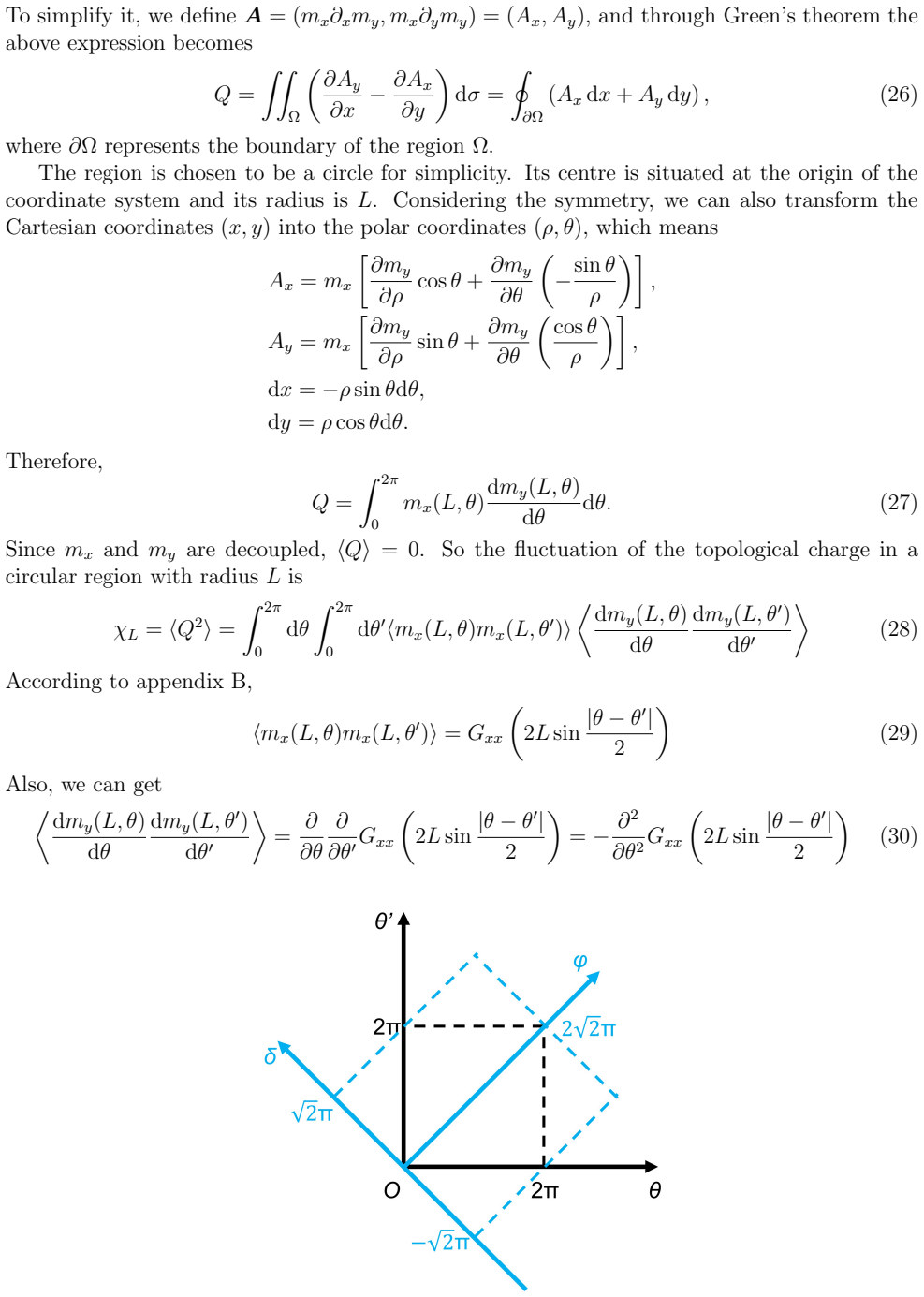
Diagram rules from Stanley [11] are stated but not proven; the whole high-T calculation depends on the enumeration and counting of these diagrams, Sections 2.1 and 2.2.1.
domain assumption At low temperatures, m_x and m_y are small fluctuations around the z-axis; the Hamiltonian and measure reduce to two decoupled massless free scalar fields, and the topological charge becomes a boundary integral of m_x d(m_y)/d(theta).
This is the load-bearing low-T assumption; no long-range order exists in 2D at any positive T, so validity is restricted to scales below the correlation length, which the paper does not discuss, Section 3, Eqs. (23)-(27).
standard math The regulator-dependent correlation function Gxx(r) has derivative G'_xx(r) = (1/(2*pi*beta*J)) (J0(r/a)-1)/r for r much smaller than the IR cutoff.
Follows from the free-field calculation with IR and UV cutoffs; the perimeter-law integral uses this derivative for arbitrarily large L by extending the upper limit to infinity, Appendix B, Eq. (51).
standard math The trace formula Tr(S_x^{2k} S_y^{2l} S_z^{2m}) = (1/(2*pi)) Gamma(k+1/2)Gamma(l+1/2)Gamma(m+1/2)/Gamma(k+l+m+3/2) is correct.
Used for all high-T coefficients; derived in Appendix A, Eq. (8)/(37).

how reviews work

0 comments

Cite this review

Pith. "Pith review of Fluctuations of topological charges in two-dimensional classical Heisenberg model through high-temperature and low-temperature expansions." pith.science (2026). https://pith.science/paper/HRWY5KEK

@misc{pith2026260803195,
  author       = {Pith},
  title        = {Pith review of: Fluctuations of topological charges in two-dimensional classical Heisenberg model through high-temperature and low-temperature expansions},
  year         = {2026},
  howpublished = {\url{https://pith.science/paper/HRWY5KEK}},
  note         = {Machine review of arXiv:2608.03195}
}

read the original abstract

It is well known that KT transition in 2d XY model is driven by the binding and unbinding of topological defects, which can be characterized by the fluctuation of topological charges inside a region. We extend the idea into the 2d Heisenberg model and calculate the fluctuation through high-temperature and low-temperature expansion respectively. It is found that the fluctuation of topological charges is proportional to the area of the region at high temperatures while obeys the perimeter law at low temperatures.

Figures

Figures reproduced from arXiv: 2608.03195 by the authors.

**Figure 1.** The lattice for calculation and the topological charge of the whole lattice is Q = P ij ρij . Similarly, the topological charge of an L × L square is QL = P 1⩽i⩽L,1⩽j⩽L ρij . Since ⟨QL⟩ = Tr QLe −βH Tr (e −βH) (10) contains odd Sij ’s, it must be zero. So the fluctuation of topological charges is χL = ⟨Q 2 L ⟩ = * X 1⩽i⩽L,1⩽j⩽L ρij!2+ . (11) Since the Hamiltonian possesses transitional invariance, the fluctuation … view at source ↗

**Figure 2.** The diagrams for the first several nonzero [PITH_FULL_IMAGE:figures/full_fig_p004_2.png] view at source ↗

**Figure 3.** The diagrams for the first several nonzero [PITH_FULL_IMAGE:figures/full_fig_p005_3.png] view at source ↗

Figures from the paper (5 more)

**Figure 4.** Figure 4: The diagrams for the first nonzero νi in ρ11rρ11l 6 [PITH_FULL_IMAGE:figures/full_fig_p006_4.png]

**Figure 5.** Figure 5: The diagrams for the first several nonzero [PITH_FULL_IMAGE:figures/full_fig_p007_5.png]

**Figure 6.** Figure 6: The diagrams for the first several nonzero [PITH_FULL_IMAGE:figures/full_fig_p008_6.png]

**Figure 7.** Figure 7: The diagrams for the first several nonzero [PITH_FULL_IMAGE:figures/full_fig_p008_7.png]

**Figure 8.** Figure 8: The graph for the coordinate transformation [PITH_FULL_IMAGE:figures/full_fig_p010_8.png]

Discussion (0). Continue with ORCID to comment.

Reference graph

Works this paper leans on

15 extracted references · 15 canonical work pages

[4]

Tang and Y

S.-C. Tang and Y. Shi, Fluctuations of topological charges in two-dimensional classical Heisenberg model. EPL149, 51001 (2025)

work page 2025
[1]

J. M. Kosterlitz and D. J. Thouless, Long range order and metastability in two dimensional solids and superfluids. (application of dislocation theory). J. Phys. C: Solid State Phys.5, L124 (1972)

work page 1972
[2]

J. M. Kosterlitz and D. J. Thouless, Ordering, metastability and phase transitions in two- dimensional systems. J. Phys. C: Solid State Phys.6, 1181 (1973)

work page 1973
[3]

J. M. Kosterlitz, The critical properties of the two-dimensional xy model. J. Phys. C: Solid State Phys.7, 1046 (1974)

work page 1974
[5]

T. H. R. Skyrme, A unified field theory of mesons and baryons. Nuclear Physics31, 556 (1962)

work page 1962
[6]

A. Fert, V. Cros and J. Sampaio, Skyrmions on the track. Nature Nanotechnology8, 152 (2013)

work page 2013
[7]

R. G. Brown and M. Ciftan, The 2d/3d classical heisenberg ferromagnet. In David P. Landau, K. K. Mon, and Heinz-Bernd Sch¨ uttler, editors,Computer Simulation Studies in Condensed-Matter Physics V, Computer Simulation Studies in Condensed-Matter Physics V, pages 150–154. Springer Berlin Heidelberg, Berlin, Heidelberg, 1993. 15

work page 1993
[8]

M. A. Klenin, Evidence for glasslike ordering in the two-dimensional classical Heisenberg magnet. Phys. Rev. B19, 4733 (1979)

work page 1979

Show all 15 references

[9]

Kawabata and A

C. Kawabata and A. R. Bishop, Monte carlo evidence for inhomogeneous states in the two-dimensional classical Heisenberg model. Solid State Commun.33, 453 (1980)

1980
[10]

Toulouse and M

G. Toulouse and M. Kl´ eman, Principles of a classification of defects in ordered media. Journal de Physique Lettres37, 149 (1976)

1976
[11]

H. E. Stanley, High-temperature expansions for the classical Heisenberg model. I. spin correlation function. Physical Review158, 537 (1967)

1967
[12]

High-temperature expansions for the classical Heisenberg model. II. zero-field susceptibility. Physical Review158, 546 (1967)

1967
[13]

H. E. Stanley and M. H. Lee, Diagrammatic representation of the two-spin correlation function for the generalized Heisenberg model. International Journal of Quantum Chemistry 4, 407 (1971)

1971
[14]

Br´ ezin and J

E. Br´ ezin and J. Zinn-Justin, Spontaneous breakdown of continuous symmetries near two dimensions. Phys. Rev. B14, 3110 (1976)

1976
[15]

Br´ ezin and J

E. Br´ ezin and J. Zinn-Justin, Renormalization of the nonlinearσmodel in 2+ϵdimensions- application to the Heisenberg ferromagnets. Phys. Rev. Lett.36, 691 (1976). 16

1976

Pith tools

Reviewed August 5, 2026 · model on record in the stance chip above.

[1] [4]

Tang and Y

S.-C. Tang and Y. Shi, Fluctuations of topological charges in two-dimensional classical Heisenberg model. EPL149, 51001 (2025)

work page 2025

[2] [1]

J. M. Kosterlitz and D. J. Thouless, Long range order and metastability in two dimensional solids and superfluids. (application of dislocation theory). J. Phys. C: Solid State Phys.5, L124 (1972)

work page 1972

[3] [2]

J. M. Kosterlitz and D. J. Thouless, Ordering, metastability and phase transitions in two- dimensional systems. J. Phys. C: Solid State Phys.6, 1181 (1973)

work page 1973

[4] [3]

J. M. Kosterlitz, The critical properties of the two-dimensional xy model. J. Phys. C: Solid State Phys.7, 1046 (1974)

work page 1974

[5] [5]

T. H. R. Skyrme, A unified field theory of mesons and baryons. Nuclear Physics31, 556 (1962)

work page 1962

[6] [6]

A. Fert, V. Cros and J. Sampaio, Skyrmions on the track. Nature Nanotechnology8, 152 (2013)

work page 2013

[7] [7]

R. G. Brown and M. Ciftan, The 2d/3d classical heisenberg ferromagnet. In David P. Landau, K. K. Mon, and Heinz-Bernd Sch¨ uttler, editors,Computer Simulation Studies in Condensed-Matter Physics V, Computer Simulation Studies in Condensed-Matter Physics V, pages 150–154. Springer Berlin Heidelberg, Berlin, Heidelberg, 1993. 15

work page 1993

[8] [8]

M. A. Klenin, Evidence for glasslike ordering in the two-dimensional classical Heisenberg magnet. Phys. Rev. B19, 4733 (1979)

work page 1979