REVIEW 3 major objections 5 minor 73 references
Confidence Horizons
T0 review · 3 major / 5 minor · reviewed 2026-08-05 · deepseek-v4-flash
Pith's one-line read This paper introduces confidence horizons: confidence sequences that are sharp on a bounded time window [m, Δm], recovering fixed-sample intervals at Δ=1 and infinite-horizon sequences as Δ→∞, with exact asymptotic coverage for means under
desk verdict Confidence horizons are a genuinely new, well-argued object — send to review, but verify the imported KMT coupling and soften the 'closed-form' claim. read the letter →
The pith
A machine-rendered reading of the paper's core claim, the machinery that carries it, and where it could break.
The reading
What carries the argument
The central object is the scaled Wiener supremum $\zeta(\Delta,q)=\sup_{s \in [1,\Delta]} |W(s)| s^{q-1}$ and its distribution $\Psi(\cdot;\Delta,q)$, whose quantile fixes the constant in front of the boundary. The argument converts the discrete-time partial-sum process into this Wiener process using distribution-uniform strong Gaussian approximation (KMT-type for independent data, Strassen’s theorem for martingales), then uses equicontinuity of $\Psi$ to make the approximation uniform in $\Delta$, $q$, and $P$. For $q \in \{0,1/2,1\}$, $\Psi$ and its one-sided version are expressed in closed form: bivariate normal integrals for $q=0,1$, and parabolic-cylinder/Ornstein–Uhlenbeck series for $q=1/2$.
What would settle it
Simulate many distributions from the stated class, including one with a moment $\kappa$ only slightly above 2, and compute worst-case coverage of the 0.95 horizon over $\Delta=3$ at $m=10^5$ using a variance estimator that satisfies Condition 3. If $\sup_P |\text{coverage} - 0.95|$ fails to shrink as $m$ grows, the uniform sharpness claim is false; a fixed-m experiment alone cannot falsify the asymptotic theorem.
Extended reading notes
Core claim
For independent data satisfying uniform moment and variance conditions, and for any variance estimator consistent at a log rate, the intervals $\hat{\mu}_t \pm \hat{\sigma}_t (m/t)^q m^{-1/2} \Psi^{-1}(1-\alpha; \Delta, q)$ form a sharp $(1-\alpha)$-asymptotic confidence horizon: $\lim_{m \to \infty} P(\forall t \in [m, \Delta m]: \mu_{P,t} \in \bar{C}_t) = 1-\alpha$, uniformly over distributions and $\Delta$ for $q \neq 1/2$, and weakly uniformly for $q=1/2$. The same guarantee holds for martingale-dependent data under almost-sure variance convergence and a Lindeberg-type uniform integrability condition. The construction is inverted to give p-values for bounded-horizon weak-null testing, and the same machinery upgrades the classical Wang–Tsiatis group sequential boundaries into
Load-bearing premise
Everything rests on the partial-sum process being uniformly close to a Wiener process with error $o_P(t^{-1/2} \log t)$ after studentization, together with a variance estimator that is consistent at a log rate; if the coupling rate or variance estimator fails, exact horizon coverage is not guaranteed.
Editorial extensions
If this is right
- At Δ=1 the confidence horizon reduces to the usual CLT interval; as Δ→∞ it approaches an asymptotic confidence sequence, so the construction continuously interpolates between fixed-sample and infinite-horizon inference.
- Analysts can peek at every time in a bounded window and stop early, getting exact asymptotic coverage instead of conservative infinite-horizon guarantees.
- Quantiles for q∈{0,1/2,1} are computed by at most one numerical integration, bypassing repeated K-dimensional integration in group sequential designs.
- Wang–Tsiatis, Pocock, and O’Brien–Fleming boundaries become continuous analogues and inherit uniform validity and martingale-dependence validity.
- In adaptive experiments under Neyman allocation, horizons separate arms and allow earlier stopping that asymptotic confidence sequences cannot.
Reading between the lines
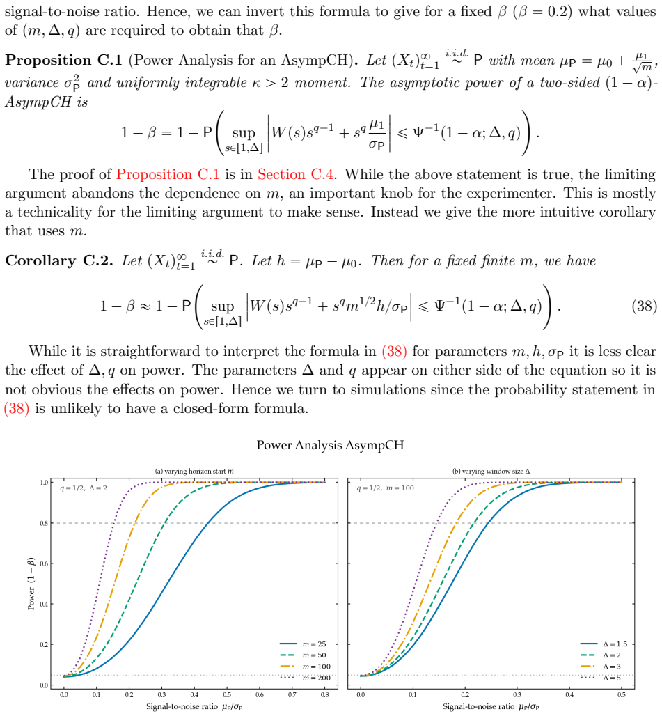
- The paper’s power analysis suggests a design rule that is only partly developed: larger q gives more end-of-window power, while q=1/2 minimizes expected stopping time, so q should be chosen by the analyst’s objective.
- The same mechanism—Gaussian coupling plus log-rate variance consistency—should extend to asymptotically linear semiparametric estimators beyond means, since only those two ingredients are used.
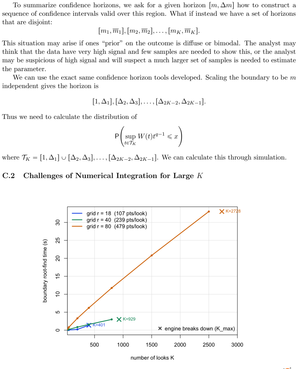
- Multiple disjoint horizons could be combined without a union bound by simulating the supremum over a union of intervals, an appendix sketch that could become a practical tool for diffuse or bimodal prior signal locations.
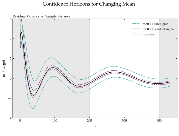
- The residual-type variance estimator recommendation for time-varying means suggests pairing confidence horizons with difference-based variance estimators in non-stationary streams.
Editorial analysis
A structured set of objections, weighed in public.
Referee Report
Summary. The paper introduces "asymptotic confidence horizons" (AsympCHs): intervals \bar C^{(m,\Delta)}_t = \hat\mu_t \pm \hat\sigma_t (m/t)^q m^{-1/2} \Psi^{-1}(1-\alpha;\Delta,q), designed to satisfy the bounded-horizon coverage guarantee lim_{m\to\infty} P(\forall t\in[m,\Delta m]: \mu_{P,t}\in\bar C_t) = 1-\alpha. The construction interpolates between fixed-sample CLT intervals (\Delta=1) and asymptotic confidence sequences (\Delta\to\infty). The main results are: Theorem 3.3 for independent, non-identically distributed data under Conditions 1-3; Theorem 3.7 for martingale-dependent data under Conditions 4-5 and Condition 3; one-sided analogues in Proposition 3.4; p-values for the weak null in Proposition 3.6; a Neyman-allocation application in Proposition 4.1; and uniformly valid group sequential analogues in Propositions 5.2 and 5.4. The proofs use strong Gaussian approximations (Lemma A.12, imported from [68], and Lemma A.13, via Strassen), followed by a continuous-time boundary-crossing analysis. Appendix B gives analytic expressions for the required quantiles for q\in\{0,1/2,1\}.
Significance. If the central result is correct, this is a useful contribution to asymptotic sequential inference. It quantifies the statistical gain from restricting validity to a finite horizon, yields explicit boundary-crossing quantiles, and provides distribution-uniform versions of both confidence horizons and group sequential methods. The paper is careful about the distinction between pointwise and uniform validity, and it is honest about finite-sample discrepancies in the Neyman-allocation simulation. The code links are a positive feature. However, the main theorem is built on an external distribution-uniform coupling whose hypotheses are not reproduced in the manuscript; the central claim is therefore conditional on an unexamined result.
major comments (3)
- [§A.2, Lemma A.12, and proof of Theorem 3.3 (§A.3.1)] The proof of Theorem 3.3 verifies Condition C2 (the additive Gaussian coupling at rate o_P(t^\gamma\log t), \gamma<-1/2) entirely by Lemma A.12, which states that [68, Corollary 3.4] implies such a coupling for sequences satisfying Conditions 1 and 2. The corollary is not stated, and its hypotheses are not checked against Conditions 1-2. This is load-bearing: Lemma A.14 replaces the empirical process by a Wiener process precisely at this step, and the sharp coverage claim of Theorem 3.3 does not follow if [68, Corollary 3.4] requires stronger or different assumptions (for example, larger moment order, i.i.d. data, or an exponential moment). The authors should state the corollary and either prove it under the stated conditions or add the required hypotheses to Theorem 3.3.
- [§3.2, Condition 3 and Variance Estimation paragraph] Theorem 3.3 is conditional on Condition 3, but the manuscript does not establish that the usual sample variance satisfies Condition 3 for independent non-identically distributed data under Conditions 1-2. The variance-estimation discussion admits that the raw sample variance may fail when the running mean varies (Eq. (13)) and recommends residual-type estimators. This is not itself an inconsistency, but the practical scope of Theorem 3.3 is narrower than the abstract's emphasis on i.i.d./independent means suggests. Please state more prominently which estimators are covered and under which additional conditions, especially in the non-i.i.d. case.
- [§5.2, Propositions 5.2 and 5.4] The claimed uniform validity of Wang-Tsiatis group sequential methods for independent and martingale-dependent data inherits the same unexamined dependency: Proposition 5.2 is proved by checking C1 and C2, and C2 is obtained from Lemma A.12 / [68, Corollary 3.4]. The discussion in Remark 5.3 emphasizes uniformity over K and over the design, which is a strong and interesting claim; the proof should make the supporting coupling theorem explicit so that the uniformity claim is verifiable.
minor comments (5)
- [Abstract and §B.2 (Remark 3.5)] The phrase "closed-form distribution functions" for q=1/2 is somewhat strong: Proposition B.4 and Lemma B.6 express the distribution through infinite series involving zeros of parabolic cylinder functions, so computing the quantile still requires root-finding. The paper should temper "closed-form" or define the sense in which these expressions are closed-form.
- [§3.2, paragraph after Theorem 3.3] For general q, the authors note that quantiles computed by Monte Carlo "may be anticonservative for any fixed level of precision." This is an important caveat for users; it would be helpful to add a recommendation about error control or interpolation between the closed-form cases.
- [§4, Fig. 5 and surrounding text] The Neyman-allocation simulation reports per-arm coverage estimates that fall slightly below 0.95 for some arms, and the text correctly attributes this to finite-sample behavior of an asymptotic guarantee. Reporting Monte Carlo standard errors would make the discrepancy easier to interpret.
- [§B.2, Lemma B.6] The notation B_\mu A_{\nu_n}(x) in Lemma B.6 is confusing: it denotes the derivative with respect to the index \mu of A_\mu(x) evaluated at \nu_n. Please clarify the notation, since this is a key quantity in the two-sided q=1/2 formula.
- [Throughout] There are occasional typos and stylistic issues (e.g., "V ariance Estimation" in the section heading, and some missing periods). A careful proofreading pass would help.
Circularity Check
No significant circularity: quantiles are Wiener-process crossing values, not fitted; the main self-cited dependency (KMT approximation from [68]) is external and does not reduce the theorem to its inputs.
full rationale
The central derivation is self-contained in the relevant sense. The quantile Ψ^{-1}(1−α; Δ, q) is defined as the inverse of the distribution of sup_{s∈[1,Δ]} |W(s)| s^{q−1} for a standard Wiener process, and Section B derives closed forms for q∈{0,1/2,1} from external Wiener/Ornstein–Uhlenbeck hitting-time results. Theorem 3.3 is proved by showing, under Conditions 1–3, that the studentized running-mean process converges uniformly to this Wiener functional (Lemma A.14) and then inverting the limiting distribution. That is a standard strong-approximation/CLT argument, not a definitional equivalence or a fit renamed as a prediction. The only author-overlapping dependency is Lemma A.12, which imports Corollary 3.4 of [68] (Waudby-Smith, Larsson, Ramdas) to obtain a distribution-uniform KMT coupling. This is load-bearing for uniformity, but it is an external, separately stated theorem with its own assumptions (moment summability and variance stability, given here as Conditions 1–2) that do not include the confidence-horizon guarantee. Under the review rules, such a citation is independent support and does not by itself constitute circularity. The manuscript does not restate the full hypotheses of [68, Cor. 3.4], which is a completeness/correctness risk rather than a circularity. The Monte Carlo remark for general q explicitly warns that simulation-based quantiles may be anticonservative, which is an honest limitation, not a fitted-input maneuver. The connections to Pocock, O’Brien–Fleming, and Wang–Tsiatis are explicitly framed as connections and the paper derives its own closed-form distributions rather than renaming the known group-sequential constants. Overall, no step reduces by construction to its inputs; the score reflects only the presence of a load-bearing but non-circular self-citation.
Assumptions & free parameters
assumptions (5)
- standard math Komlós-Major-Tusnády strong approximation holds uniformly over P at the stated rate (Lemma A.12, using [68, Cor. 3.4]).
- standard math Strassen's strong approximation for martingales holds under Condition 4 and 5 (Lemma A.13, [57]).
- standard math The distribution functions F and F_+ are equicontinuous and invertible on the needed domains (Lemma A.4, A.8).
- domain assumption Moment conditions Condition 1, 2, and variance estimator consistency Condition 3 for independent data; Conditions 4 and 5 for martingale data.
- domain assumption The target parameter is the running mean \tilde{μ}_{P,t}, not a fixed parameter, for non-identically distributed data.
Cite this review
Pith. "Pith review of Confidence Horizons." pith.science (2026). https://pith.science/paper/6LGXV2WW
@misc{pith2026260803889,
  author       = {Pith},
  title        = {Pith review of: Confidence Horizons},
  year         = {2026},
  howpublished = {\url{https://pith.science/paper/6LGXV2WW}},
  note         = {Machine review of arXiv:2608.03889}
}
read the original abstract
Anytime-valid inference enables analysts to continuously monitor their data and stop experiments early. However, the majority of these methods incur a certain conservativeness by remaining valid on infinite time horizons. In practice, a bound on the horizon may be imposed due to budgetary, practical, or ethical constraints. In this paper, we ask the question: "Is it possible to obtain sharper large-sample anytime-valid inference by forgoing validity beyond some finite time horizon?". We provide a positive answer to this question by proposing a family of statistical objects that we call "confidence horizons". These objects can be viewed as large-sample confidence sequences on bounded time horizons, or alternatively as group sequential repeated confidence intervals with a maximal number of interim peeking times. We make explicit connections to the group sequential boundaries of Pocock [1977], O'Brien--Fleming [1979], and Wang--Tsiatis [1987]. We derive closed-form distribution functions of certain statistics which can be used to calculate the asymptotic quantiles of confidence horizons exactly, sidestepping the repeated integration typically employed in group sequential methods. We illustrate the use of confidence horizons for treatment effect estimation in sequentially randomized experiments under adaptive Neyman allocation.
Figures


Figures from the paper (15 more)





Reference graph
Works this paper leans on
-
[68]
I. Waudby-Smith, M. Larsson, and A. Ramdas. Nonasymptotic and distribution-uniform Koml´ os-Major-Tusn´ ady approximation.arXiv preprint arXiv:2502.06188, 2025. 35
arXiv 2025
-
[1]
S. Agrawal and A. Ramdas. On stopping times of power-one sequential tests: Tight lower and upper bounds.arXiv preprint arXiv:2504.19952, 2025. 61
arXiv 2025
- [2]
-
[3]
Anderson.gsDesign: Group Sequential Design, 2026
K. Anderson.gsDesign: Group Sequential Design, 2026. URL https://keaven.github.io/ gsDesign/. R package version 3.11.0.9003. 18
work page 2026
-
[4]
P. Armitage, C. McPherson, and B. Rowe. Repeated significance tests on accumulating data. Journal of the Royal Statistical Society: Series A (General), 132(2):235–244, 1969. 18
work page 1969
-
[5]
R. R. Bahadur and L. J. Savage. The Nonexistence of Certain Statistical Procedures in Nonparametric Problems.The Annals of Mathematical Statistics, 27(4):1115–1122, Dec. 1956. 5
work page 1956
-
[6]
R. Bellman and T. Harris. Recurrence times for the Ehrenfest model.Pacific Journal of Mathematics, 1951. 10
work page 1951
-
[7]
A. C. Berry. The accuracy of the Gaussian approximation to the sum of independent variates. Transactions of the American Mathematical Society, 49(1):122–136, 1941. 23 24
work page 1941
Show all 73 references
-
[8]
Besag and P
J. Besag and P. Clifford. Sequential Monte Carlo p-values.Biometrika, 78(2):301–304, 1991. 15
1991
-
[9]
Bibaut, N
A. Bibaut, N. Kallus, and M. Lindon. Near-optimal non-parametric sequential tests and confidence sequences with possibly dependent observations.arXiv preprint arXiv:2212.14411,
-
[10]
Blanchet-Scalliet, D
C. Blanchet-Scalliet, D. Dorobantu, and L. Gay. Joint law of an Ornstein–Uhlenbeck process and its supremum.Journal of Applied Probability, 57(2):541–558, 2020. 52
2020
-
[11]
Blanchet-Scalliet, D
C. Blanchet-Scalliet, D. Dorobantu, and B. Nieto. A pseudo-likelihood estimator of the Ornstein–Uhlenbeck parameters from suprema observations.Statistical Inference for Stochastic Processes, 27(2):407–425, 2024. 10, 51, 52
2024
-
[12]
Blanchet-Scalliet, D
C. Blanchet-Scalliet, D. Dorobantu, and B. Nieto. On the distribution of the first exit time from an interval of a threshold Ornstein-Uhlenbeck process. 2025. 10, 51, 54
2025
-
[13]
V. I. Bogachev.Gaussian measures. Number 62. American Mathematical Soc., 1998. 47
1998
-
[14]
L. Breiman. First exit times from a square root boundary. InProceedings of the Fifth Berkeley Symposium on Mathematical Statistics and Probability, Volume 2: Contributions to Probability Theory, Part 2, volume 5, pages 9–17. University of California Press, 1967. 10
1967
-
[15]
Chugg, E
B. Chugg, E. Gauthier, M. I. Jordan, A. Ramdas, and I. Waudby-Smith. Post-hoc large-sample statistical inference.arXiv preprint arXiv:2603.08002, 2026. 4
2026
-
[16]
Clerico, T
E. Clerico, T. Wegel, I. Azangulov, and P. Rebeschini. Time-sensitive anytime-valid testing. arXiv preprint arXiv:2605.06521, 2026. 4
2026 arXiv
-
[17]
T. Cook, A. Mishler, and A. Ramdas. Semiparametric efficient inference in adaptive experiments. InCausal Learning and Reasoning, pages 1033–1064. PMLR, 2024. 13, 15
2024
-
[18]
Csorgo and P
M. Csorgo and P. Revesz. How Big are the Increments of a Wiener Process?The Annals of Probability, 7(4):731–737, Aug. 1979. 44
1979
-
[19]
J. Dai, P. Gradu, and C. Harshaw. Clip-ogd: An experimental design for adaptive neyman allocation in sequential experiments.Advances in Neural Information Processing Systems, 36: 32235–32269, 2023. 13, 14
2023
-
[20]
D. A. Darling and H. Robbins. Iterated logarithm inequalities.Proceedings of the National Academy of Sciences, 57(5):1188–1192, 1967. 61
1967
-
[21]
D. A. Darling and A. J. F. Siegert. The First Passage Problem for a Continuous Markov Process.The Annals of Mathematical Statistics, 24(4):624–639, Dec. 1953. 10
1953
-
[22]
D. M. De Long. Crossing probabilities for a square root boundary by a Bessel process. Communications in Statistics-Theory and Methods, 10(21):2197–2213, 1981. 10
1981
-
[23]
J. L. Doob. The Brownian movement and stochastic equations.Annals of mathematics, 43(2): 351–369, 1942. 52
1942
-
[24]
C.-G. Esseen. On the Liapunoff limit of error in the theory of probability, 1942. 23
1942
-
[25]
Fischer and A
L. Fischer and A. Ramdas. Sequential Monte Carlo testing by betting.Journal of the Royal Statistical Society Series B: Statistical Methodology, 87(4):1200–1220, 2025. 15 25
2025
-
[26]
Hadad, D
V. Hadad, D. A. Hirshberg, R. Zhan, S. Wager, and S. Athey. Confidence intervals for policy evaluation in adaptive experiments.Proceedings of the national academy of sciences, 118(15),
-
[27]
P. Hall, J. Kay, and D. Titterington. Asymptotically optimal difference-based estimation of variance in nonparametric regression.Biometrika, 77(3):521–528, 1990. 11
1990
-
[28]
Hoeffding
W. Hoeffding. Probability inequalities for sums of bounded random variables.Journal of the American statistical association, 58(301):13–30, 1963. 5
1963
-
[29]
S. R. Howard, A. Ramdas, J. McAuliffe, and J. Sekhon. Time-uniform, nonparametric, nonasymptotic confidence sequences.The Annals of Statistics, 49(2):1055–1080, 2021. 5, 6, 22
2021
-
[30]
Imbens, L
G. Imbens, L. Masoero, A. Rakhlin, T. S. Richardson, and S. Vijaykumar. Demonstration Experiments.arXiv preprint arXiv:2603.06941, 2026. 9
2026 arXiv
-
[31]
Jennison and B
C. Jennison and B. W. Turnbull. Interim analyses: the repeated confidence interval approach. Journal of the Royal Statistical Society Series B: Statistical Methodology, 51(3):305–334, 1989. 4
1989
-
[32]
Jennison and B
C. Jennison and B. W. Turnbull. Distribution theory of group sequential t, χ2 and F-tests for general linear models.Sequential Analysis, 16(4):295–317, 1997. 4, 18
1997
-
[33]
Jennison and B
C. Jennison and B. W. Turnbull. Group-sequential analysis incorporating covariate information. Journal of the American Statistical Association, 92(440):1330–1341, 1997. 18
1997
-
[34]
Jennison and B
C. Jennison and B. W. Turnbull.Group Sequential Methods with Applications to Clinical Trials. Chapman and Hall/CRC, 2000. 3, 17, 18, 19
2000
-
[35]
M. Kato, T. Ishihara, J. Honda, and Y. Narita. Efficient adaptive experimental design for average treatment effect estimation.arXiv preprint arXiv:2002.05308, 2020. 13, 14, 15, 16, 59
2002 arXiv
-
[36]
Koml´ os, P
J. Koml´ os, P. Major, and G. Tusn´ ady. An approximation of partial sums of independent R V’s, and the sample DF. II.Zeitschrift f¨ ur Wahrscheinlichkeitstheorie und Verwandte Gebiete, 34 (1):33–58, 1976. 35
1976
-
[37]
N. W. Koning and S. Van Meer. Anytime validity is free: inducing sequential tests.Journal of the Royal Statistical Society Series B: Statistical Methodology, page qkag050, 2026. 4
2026
-
[38]
Lamperti
J. Lamperti. Semi-stable stochastic processes.Transactions of the American mathematical Society, 104(1):62–78, 1962. 52
1962
-
[39]
K. G. Lan and D. L. DeMets. Discrete sequential boundaries for clinical trials.Biometrika, pages 659–663, 1983. 18, 59
1983
-
[40]
Lattimore and C
T. Lattimore and C. Szepesv´ ari.Bandit algorithms. Cambridge University Press, 2020. 14
2020
-
[41]
Liang and I
B. Liang and I. Bojinov. An experimental design for anytime-valid causal inference on multi- armed bandits.arXiv preprint arXiv:2311.05794, 2023. 14
2023 arXiv
-
[42]
Marcinkiewicz and A
J. Marcinkiewicz and A. Zygmund. Sur les fonctions ind´ ependantes.Fundamenta Mathematicae, 29:60–90, 1937. 12 26
1937
-
[43]
Massiani, S
P.-F. Massiani, S. Schulze, and M. Mollenhauer. Asymptotic e-processes.arXiv preprint arXiv:2604.19353, 2026. 4
2026 arXiv
-
[44]
McDiarmid and others
C. McDiarmid and others. On the method of bounded differences.Surveys in combinatorics, 141(1):148–188, 1989. 5
1989
-
[45]
M¨ orters and Y
P. M¨ orters and Y. Peres.Brownian motion, volume 30. Cambridge University Press, 2010. 44, 56
2010
-
[46]
Neopane, A
O. Neopane, A. Ramdas, and A. Singh. Logarithmic neyman regret for adaptive estimation of the average treatment effect.arXiv preprint arXiv:2411.14341, 2024. 13
2024 arXiv
-
[47]
J. Neyman. On the Application of Probability Theory to Agricultural Experiments. Essay on Principles. Section 9 (translated, reprinted ed.).Statistical Science, 5(4):465–472, 1923. 13, 14
1923
-
[48]
J. Neyman. On the Two Different Aspects of the Representative Method: The Method of Stratified Sampling and the Method of Purposive Selection.Journal of the Royal Statistical Society, 97(4):558–625, 1934. 13
1934
-
[49]
P. C. O’Brien and T. R. Fleming. A multiple testing procedure for clinical trials.Biometrics, 35(3):549–556, 1979. 4, 6, 17, 20, 24
1979
-
[50]
S. J. Pocock. Group sequential methods in the design and analysis of clinical trials.Biometrika, 64(2):191–199, 1977. 4, 6, 17, 18, 20, 24
1977
-
[51]
Ramdas and R
A. Ramdas and R. Wang. Hypothesis testing with e-values.Foundations and Trends®in Statistics, 1(1-2):1–390, 2025. 61
2025
-
[52]
H. Robbins. Statistical methods related to the law of the iterated logarithm.The Annals of Mathematical Statistics, 41(5):1397–1409, 1970. 6
1970
-
[53]
Robbins and D
H. Robbins and D. Siegmund. Boundary crossing probabilities for the Wiener process and sample sums.The Annals of Mathematical Statistics, pages 1410–1429, 1970. 1, 5
1970
-
[54]
D. B. Rubin. Estimating causal effects of treatments in randomized and nonrandomized studies. Journal of educational Psychology, 66(5):688, 1974. 13, 14
1974
-
[55]
D. O. Scharfstein, A. A. Tsiatis, and J. M. Robins. Semiparametric efficiency and its implication on the design and analysis of group-sequential studies.Journal of the American Statistical Association, 92(440):1342–1350, Dec. 1997. 18
1997
-
[56]
W. F. Stout. The Hartman-Wintner law of the iterated logarithm for martingales.The Annals of Mathematical Statistics, 41(6):2158–2160, 1970. 12
1970
-
[57]
Strassen
V. Strassen. Almost sure behavior of sums of independent random variables and martingales. Proceedings of the Fifth Berkeley Symposium on Mathematical Statistics and Probability, 3,
-
[58]
E. O. Taga, S. Oymak, and S. Shekhar. Learning to bet for horizon-aware anytime-valid testing. arXiv preprint arXiv:2603.19551, 2026. 4
2026 arXiv
-
[59]
A. A. Tsiatis, H. Boucher, and K. Kim. Sequential methods for parametric survival models. Biometrika, 82(1):165–173, 1995. 18 27
1995
-
[60]
A. W. Van Der Vaart, J. H. Van Zanten, and others. Reproducing kernel Hilbert spaces of Gaussian priors.IMS Collections, 3:200–222, 2008. 30
2008
-
[61]
Vor´ acek and F
V. Vor´ acek and F. Orabona. STaR-Bets: Sequential target-recalculating bets for tighter confidence intervals.Advances in Neural Information Processing Systems, 38:161909–161953,
-
[62]
A. Wald. Sequential Tests of Statistical Hypotheses.The Annals of Mathematical Statistics, 16 (2):117 – 186, 1945. 61
1945
-
[63]
S. K. Wang and A. A. Tsiatis. Approximately optimal one-parameter boundaries for group sequential trials.Biometrics, pages 193–199, 1987. 17, 18, 19, 20, 21
1987
-
[64]
Waudby-Smith and A
I. Waudby-Smith and A. Ramdas. Estimating means of bounded random variables by betting. Journal of the Royal Statistical Society Series B: Statistical Methodology, 86(1):1–27, 02 2024. 4
2024
-
[65]
Waudby-Smith, E
I. Waudby-Smith, E. H. Kennedy, and A. Ramdas. Distribution-uniform anytime-valid sequential inference and the robbins-siegmund distributions.arXiv preprint arXiv:2311.03343, 2023. 1, 2, 3, 4, 5, 10, 29, 31, 37, 43
2023
-
[66]
Waudby-Smith, D
I. Waudby-Smith, D. Arbour, R. Sinha, E. H. Kennedy, and A. Ramdas. Time-uniform central limit theory and asymptotic confidence sequences.The Annals of Statistics, 52(6):2613–2640,
-
[67]
Waudby-Smith, M
I. Waudby-Smith, M. Larsson, and A. Ramdas. Distribution-uniform strong laws of large numbers.arXiv preprint arXiv:2402.00713, 2024. 9
2024 arXiv
-
[69]
1and supT“ ∆. Then @εą 0, there exists anη
I. Waudby-Smith, R. Sandoval, and M. I. Jordan. Universal log-optimality for general classes of e-processes and sequential hypothesis tests.arXiv preprint arXiv:2504.02818, 2025. 61 28 A Proofs of the Main Results We use the stochastic ¯onotation suggested in Waudby-Smith et a...
2025 arXiv
-
[71]
´c 2 and the “canonical
If Xp0q„Np0,1q, then P ˜ sup sPr1,∆s |Wpsq|s ´1{2ěx ¸ “ ż x ´8 Pz ˜ sup tPr0,log ∆{2s |Xptq|ěx ¸ ϕpzqdz`Φp´xq, and P ˜ sup sPr1,∆s Wpsqs´1{2ěx ¸ “ ż x ´8 Pz ˜ sup tPr0,log ∆{2s Xptqěx ¸ ϕpzqdz`Φp´xq. Therefore, finding distribution functions for q“ 1{2 amounts to finding them ...
-
[72]
First, recall a property ofA µpyq
This leaves us with G0,µpx, yq“B µpyqAµpxq´B µpxqAµpyq, where Bµpyq“ y? 2 M ˆ 1´µ 2 ; 1.5; y2 2 ˙ , and Aµpyq“M ˆ´µ 2 ; 0.5; y2 2 ˙ , whereMis the hypergeometric (Kummer’s) function. First, recall a property ofA µpyq. Lemma B.7.LetA µpyq“Mp ´µ 2 ; 0.5; y2 2q. d dy Aµpyq“´µyM ˆ...
-
[73]
power-one
Therefore, the correlation of the two random variables is´c 1{ a 1`c 2 1 and we can write PpU´c 1Xďc 2, Xăaq´PpU´c 1Xďc 2, Xă´aq“P ´ rUďc 2, Xăa ¯ ´P ´ rUďc 2, Xă´a ¯ “Φ 2 ˜ c2a 1`c 2 1 , a; ´c1a 1`c 2 1 ¸ ´Φ 2 ˜ c2a 1`c 2 1 ,´a; ´c1a 1`c 2 1 ¸ Lemma B.10.LetD νp¨qbe the parab...
-
[2024]
1, 2, 3, 4, 5, 6, 9, 22, 36
Reviewed August 5, 2026 · model on record in the stance chip above.
Discussion (0). Sign in to comment.