Stability of Differential Stochastic Variational Inequalities with History-Dependent Responses and Transfer Learning

Guan Wang; Jian Guo; Xiaojun Chen; Xin Guo

REVIEW 2 major objections 3 minor 43 references

Stability of Differential Stochastic Variational Inequalities with History-Dependent Responses and Transfer Learning

T0 review · 2 major / 3 minor · reviewed 2026-08-10 · deepseek-v4-flash

Challenge this review Re-run · record.json Download PDF Read on arXiv ↗ Review JSON

Pith's one-line read Two similar stochastic environments produce close trajectories, the paper proves, giving a quantitative license for transfer learning in history-dependent differential stochastic variational inequalities.

desk verdict Genuine extension of DSVI theory with a useful transfer-stability bound, but the main theorem's quantitative content is conditional on a finiteness assumption that is hidden in a definition rather than stated as a hypothesis. read the letter →

arxiv 2608.06923 v1 pith:JQLGIZSF submitted 2026-08-07 math.OC

Xiaojun Chen , Jian Guo , Xin Guo , Guan Wang This is my paper · ORCID

classification math.OC MSC 90C1590C3390C39

keywords differentialstochasticvariationalinequalityhistory-dependentresponsetransferlearningsampleaverageapproximationWassersteinstabilityparametricmovingfeasiblesetelderlyhealthmonitoring

verification ladder T0 review T1 audit T2 compute T3 formal

The pith

A machine-rendered reading of the paper's core claim, the machinery that carries it, and where it could break.

The reading

This paper proposes a class of history-dependent differential stochastic variational inequalities (DSVIs): an ordinary differential equation whose drift is the expected value of a feedback mapping involving a response defined by a variational inequality over the entire past path of an exogenous random process. It establishes that these systems are well posed — the stochastic response is unique, measurable, and Lipschitz in the current state, so the coupled trajectory exists and is unique — and that sample-average approximations of the drift converge uniformly almost surely. Its central result is a transfer-stability theorem: two such systems with different initial states and different laws for the exogenous process produce trajectories whose uniform distance is bounded by the initial-state difference plus the Wasserstein distance between the path laws and the square root of that distance. Because the bound is explicit and quantitative, it gives a theoretical justification for reusing responses computed in one stochastic environment as approximations in another similar one. The paper closes with an elderly-health monitoring case study in which similarity-weighted reuse of precomputed responses reaches accuracy close to the full-recomputation benchmark while cutting online batch runtime from 86 seconds to under one second.

What carries the argument

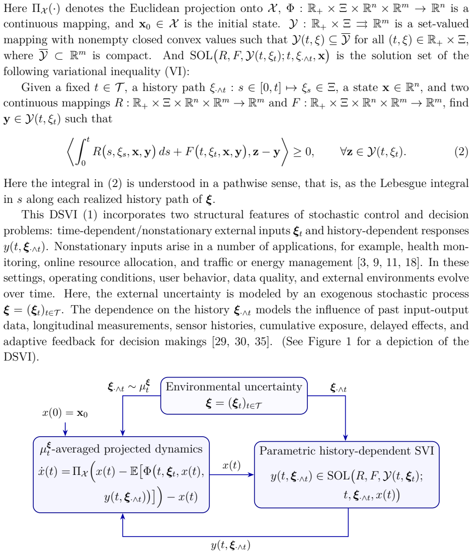
The load-bearing object is the history-dependent map $\Psi(t,\xi_{\cdot\wedge t},x,y) = \int_0^t R(s,\xi_s,x,y)\,ds + F(t,\xi_t,x,y)$, whose unique zero defines the second-stage response $y(t,\xi_{\cdot\wedge t},x)$ as the solution of a parametric variational inequality over the moving feasible set $Y(t,\xi_t)$. Under strong monotonicity of $F$ with constant $m_F > 0$ and Lipschitz problem data, the response is unique, measurable, and Lipschitz in the state; under a Hausdorff-Lipschitz assumption on the feasible-set map, the response changes by at most $C_Y(t)\big(\|\xi^\alpha - \xi^\beta\|_\infty + \|\xi^\alpha - \xi^\beta\|_\infty^{1/2}\big)$ between two histories. That square-root rate is carried through the expectation over path laws and integrated via Gronwall's inequality, which is how the theorem's $W_1 + W_1^{1/2}$ trajectory bound emerges.

What would settle it

Fix identical initial states and drive the Wasserstein distance $W_1(\mu^\alpha,\mu^\beta)$ to zero while measuring $\sup_{t \in [0,T]}\|x^\alpha(t) - x^\beta(t)\|$: Theorem 6 requires this error to decay at least as fast as a constant times $W_1 + \sqrt{W_1}$, so an experiment showing the error stays bounded away from zero as $W_1 \to 0$, or decays at a strictly slower rate, would refute the bound. A crisp construction would embed the corner-tip feasible sets of the paper's Example 1 into the second stage and let the two path laws differ only in how often the path touches the corner.

Watch

Extended reading notes

Core claim

The paper's central discovery is Theorem 6: for two history-dependent DSVIs with identical data — same mappings $R$, $F$, $\Phi$, same constraint sets, same horizon — but different initial states $x_0^\alpha$, $x_0^\beta$ and different exogenous path laws $\mu^\alpha$, $\mu^\beta$, the first-stage trajectories satisfy $$\|x^\$\alpha$ - x^\$\beta$\|_\infty \le C_T\left(\|x_0^\$\alpha$ - x_0^\$\beta$\| + W_1(\mu^\$\alpha$,\mu^\$\beta$) + W_1(\mu^\$\alpha$,\mu^\$\beta$)^{1/2}\right),$$ with a finite constant $C_T$ assembled from the regularity constants and the horizon. The exponent $1/2$ is not an artifact: a constructed example shows that feasible sets moving Lipschitz-continuously in Hausdorff distance can force the variational-inequality response to be only square-root-Hölder continuous in the path, and this rate propagates from the second-stage response through the drift to the trajectory. The paper reads this as a quantitative license for transfer learning: similar source and target environments and initial states yield close trajectories, so precomputed response trajectories from a source system can be reused for a target system with a controlled, explicit error.

Load-bearing premise

The argument rests on $F$ being strongly monotone in the response variable with a fixed positive constant $m_F$, which drives uniqueness of the response and every quantitative estimate, and on the response operator $\Psi$ being uniformly bounded over all histories and states so that $M_\Psi(t)$ is finite; if either premise fails, the stability and transfer bounds weaken or become vacuous.

Editorial extensions

If this is right

Transfer learning across history-dependent DSVI systems carries a provable error certificate: when source and target differ by small initial-state and Wasserstein distances, the reused trajectory is close in uniform norm with the explicit constant $C_T$.
The $1/2$-Hölder rate tells practitioners to expect transfer error to shrink like the square root of the environment distance whenever feasible sets move with the environment, not linearly.
Sample-average approximation of the drift converges uniformly almost surely, so finite-sample computations faithfully approximate the exact expected-value dynamics as the sample size grows.
Response trajectories can be reused across time as well as users: refresh intervals of several minutes hold accuracy near the full-update benchmark while cutting recomputation cost by an order of magnitude.
In the elderly-health monitoring application, similarity-weighted reuse of precomputed responses reaches accuracy near the 97 percent full-recomputation benchmark while cutting online batch runtime from 86 seconds to about 0.62 seconds.

Reading between the lines

Editorial extensions of the paper, not claims the author makes directly.

The square-root term in Theorem 6 is plausibly sharp: because the paper's own Example 1 shows a Hausdorff-Lipschitz moving feasible set can force exactly $1/2$-Hölder response behavior, transfer error proportional to $\sqrt{W_1}$ near nonsmooth feasible-set changes is likely unavoidable without extra structure.
A design principle follows that the paper leaves implicit: engineer the second-stage feasible set to vary smoothly, or precompute responses on a fixed grid of feasible sets, to convert the $1/2$-Hölder factor into a linear one and tighten the transfer bound.
Because the bound needs $\sup\|\Psi\|$ over all histories and states, it is vacuous for unbounded state spaces; replacing the supremum by an $L^p$ moment of $\Psi$ under the path law would plausibly extend the transfer guarantee to unbounded systems.
The 139-fold latency reduction suggests the dominant online cost in such monitoring systems is second-stage response recomputation, so caching and similarity-weighted lookup are the effective levers for real-time deployment; this is worth confirming on non-synthetic cohorts.

Share X Bluesky LinkedIn Reddit HN

Signed reviews

No signed human review yet.

Editorial analysis

A structured set of objections, weighed in public.

Desk editor's note, referee report, and a circularity audit.

Desk Editor's Note

read the letter

Bottom line: this is a real contribution, and the transfer-stability bound is worth publishing, but the main theorem is stated more broadly than the assumptions support. The paper's new content is genuine: a DSVI whose second-stage VI depends on the full history through the integral term involving R, reducing to the earlier models in [10, 11, 14] when R = 0; a well-posedness result built on strong monotonicity and Carathéodory ODE theory; an SAA convergence theorem; and a 1/2-Hölder stability estimate for parametric VIs with Hausdorff-Lipschitz moving feasible sets, leading to a trajectory bound in Wasserstein distance. The proofs are detailed and, as far as I checked, correct. The 1/2-Hölder exponent is not an artifact: the moving-set example in Section 4.2 shows why Lipschitz continuity fails, and the exponent is natural there.

The load-bearing soft spot is Lemma 5. The constant CY(t) is defined using MΨ(t) = sup ||Ψ||, and finiteness of MΨ(t) is asserted as part of the definition rather than listed as a hypothesis. Theorem 6 then needs ∫ sqrt(MΨ(t)) dt < ∞ for CT to be finite. Assumption 1 does not imply this: R is bounded only on compact x-sets and F is only Lipschitz in ξ, so with X or Ξ unbounded the supremum is typically infinite. A concrete counterexample: R = 0, F(t,ξ,x,y) = y + ξ, Y(t,ξ) = [−1,1]^m, X = Ξ = R^n satisfies A1–A2 and Hausdorff-Lipschitz Y, yet MΨ(t) = ∞ and both CY and CT blow up. The numerical experiments use compact X = [0,2] and bounded features, so the application is safe, but the theorem as stated is vacuous outside such cases. This is fixable: state explicitly that X and Ξ are compact (or that MΨ is finite with the needed integrability) and adjust the theorem statements accordingly.

Minor issues: strong monotonicity with m_F > 0 drives all bounds; that is a real limitation but a standard one. The abstract's 'benchmark of 0.97' is sloppy against Table 5's 97.928%, and the health-monitoring experiments are synthetic with no error bars; the authors do note the noise-robustness study is one user. None of these change the theoretical contribution.

Who this is for: researchers working on differential stochastic variational inequalities, stochastic generalized equations, or transfer learning in dynamic systems. The theory is solid enough to warrant a serious referee. I would send it out, with a request to fix the finiteness hypothesis and tighten the numerics.

Referee Report

2 major / 3 minor

Summary. The paper introduces a class of history-dependent differential stochastic variational inequalities (DSVIs) in which a projected ODE is coupled to a stochastic variational inequality whose data include the history of an exogenous process. Section 2 establishes existence, uniqueness, measurability, and state-Lipschitz continuity of the second-stage response, and hence well-posedness of the closed-loop trajectory under strong monotonicity, Lipschitz, and integrability conditions. Section 3 develops a sample average approximation of the expected drift and proves uniform almost-sure convergence of the approximate state trajectories. Section 4 contains the principal novelty: a local 1/2-Hölder estimate for parametric VIs with Hausdorff-Lipschitz moving feasible sets and a transfer-stability bound for first-stage trajectories in terms of the initial-state difference and the Wasserstein distance between exogenous path laws. Sections 5 and 6 provide numerical experiments on SAA convergence, source-to-target transfer stability, and an elderly-health monitoring application, where similarity-weighted reuse of source responses nearly matches the target-domain full-recomputation baseline while sharply reducing online latency.

Significance. If the theorems hold as stated, the paper is a useful contribution: it unifies several earlier DVI/SVI models, gives detailed existence and SAA proofs with explicit constants, and formulates a quantitative transfer-learning statement for a control-theoretic setting. The authors are careful to express all constants in Theorems 2, 4, and 6 through assumed quantities such as m_F, ℓ_F, ℓ_R, and W1 rather than fitted parameters, and the numerical study is reproducible via a linked repository. The paper also states limitations, including the single-user noise-robustness study and the exclusion of offline precomputation from the reported online runtime. The main caveat is that the transfer-stability theorem currently rests on an unstated global boundedness/integrability condition; once that condition is made explicit, the results would be a solid contribution to the DSVI and transfer-learning literature.

major comments (2)

[§4.2–4.3, Lemma 5 and Theorem 6] The transfer-stability result depends critically on the quantity MΨ(t), but its finiteness is asserted inside the definition of CY(t) in Lemma 5 rather than stated as a hypothesis, and Theorem 6 does not list any boundedness condition on X or Ξ that would imply it. Assumption 1 does not imply MΨ(t)<∞: for example, take X=R^n, Ξ=R^m, R≡0, F(t,ξ,x,y)=y+ξ, and Y(t,ξ)≡[-1,1]^m; then Assumption 1(A1)-(A2) and the Hausdorff-Lipschitz condition on Y hold, yet MΨ(t)=sup_{ξ∈R^m, y∈[-1,1]^m} ||y+ξ||=∞. Moreover, the proof of Theorem 6 needs not only pointwise finiteness of MΨ(t) but also integrability of sqrt(MΨ(t)) on [0,T], since D(t)=ℓΦ(t)(1+CY(t)) enters CT through ∫_0^T D(s)ds. Please add an explicit compactness or boundedness assumption on X and Ξ, or replace MΨ(t) by a local bound, and state the corresponding integrability condition as a hypothesis of Lemma 5 and Theorem 6.
[§3, Theorem 4] The statement of Theorem 4 says 'Suppose that the assumptions of Theorem 2 hold', but its proof invokes Lemma 3, which additionally requires X to be compact. The paragraph before Lemma 3 states that compactness of X is assumed for the SAA convergence analysis, so this is likely intended as a standing assumption for Section 3; nevertheless, Theorem 4 as printed should include it explicitly. Otherwise the theorem statement is formally weaker than its hypotheses, and the SAA convergence claim is not justified without compactness.

minor comments (3)

[Example 1, §4.2] The notation qε=(ε,pε) is inconsistent with the displayed projection formula: the bound ||yε-y0||=sqrt(ε/(1+ε)) holds only if pε=√ε. Please define pε=√ε or write qε=(ε,√ε) explicitly.
[§6.2.1] The transfer experiments measure source-target similarity by feature-space distances d(v,u), whereas Theorem 6 is formulated in terms of W1 between full path laws. The connection between the theorem and the numerical transfer procedure is therefore heuristic; the text should acknowledge this gap rather than presenting the experiment as a direct instantiation of Theorem 6.
[Abstract and Table 5] The abstract says the transfer accuracy is 'close to the full-recomputation benchmark of 0.97', while Table 5 reports the full-recomputation baseline as 97.928% accuracy. The rounding to 0.97 is slightly loose; consider reporting 0.979 or writing 'over 0.97' to avoid an apparent inconsistency.

Circularity Check

0 steps flagged · score 1.0 of 10

No significant circularity: the SAA and transfer-stability theorems are proven from explicit assumptions, and the self-citations are background or special cases rather than load-bearing evidence.

full rationale

I walked the derivation chain from Assumption 1 through Lemma 1, Theorem 2, Lemma 3, Theorem 4, Lemma 5, and Theorem 6, and also checked the numerical sections. No step defines a target quantity in terms of itself, and no fitted parameter is relabeled as a prediction. The constants in the main results, such as kappa_Y(t), beta(t), C_Y(t), and C_T, are explicit functions of the assumed data (m_F, l_F, l_R, l_Phi, L_Y, M_Psi, and T); they are never calibrated from the experiments. Lemma 1 proves uniqueness and Lipschitz continuity from strong monotonicity, Theorem 2 uses a standard Caratheodory ODE existence theorem, Lemma 5 derives the 1/2-Holder estimate using the variational inequality and strong monotonicity, and Theorem 6 combines Lemma 5 with Gronwall's inequality. The transfer-learning application in Section 6 is an engineering evaluation with its own similarity weights and held-out labels; it does not feed fitted constants back into Theorem 6. The citations to the authors' prior work, especially [10,11,14,17,27], are used as background, as special cases, or as related convergence results, but not as the justification for the central stability claim. The only notable concern is technical rather than circular: Lemma 5 states M_Psi(t) < infinity inside the definition of C_Y(t), effectively imposing an unstated boundedness condition that can fail for unbounded X or Xi and would make C_T infinite. This is a robustness or correctness gap, not a circularity of the derivation.

Assumptions & free parameters 3 free parameters · 10 assumptions · 0 invented entities

The central theory rests on standard strong-monotonicity, Lipschitz, and measurability assumptions, plus a less-clearly-stated finiteness condition on M_Psi. No new physical entities are introduced. The numerical experiments introduce hand-chosen constants that affect the application results but are not used in the theoretical derivations.

free parameters (3)

K (number of source users in transfer) = 8
The mean transfer accuracy is maximized at K=8 in Table 4; the authors select this value for the headline speedup and accuracy comparison.
lambda_i and rho_i in health-monitoring response = lambda_i=0.50, rho_i=5 for i=1,2,3
Hand-chosen weights in the response objective in Section 6.1; they balance historical fitting and current-state consistency.
synthetic dynamics constants = A(t)=exp(-3), p(t)=0.01, q(t) coefficients, l0=0.02, Delta l1=1.5, alpha=(0.4,0.4,0.2)
Chosen by hand to emulate damage-repair and circadian dynamics in the synthetic health benchmark; not fitted to the theory.

assumptions (10)

domain assumption Assumption 1(A1): R(t, xi, x, .) is monotone, Lipschitz in (xi, x, y) with integrable modulus, and bounded uniformly on compact x-sets.
Used in Lemma 1 to get strong monotonicity of Psi and Lipschitz dependence of the response on x.
domain assumption Assumption 1(A2): F is strongly monotone in y with constant m_F > 0 and Lipschitz in (xi, x, y).
Provides the m_F > 0 that drives uniqueness and all subsequent quantitative bounds.
domain assumption Assumption 1(A3): Phi is Lipschitz with integrable modulus and growth bound b_Phi(t, xi_t).
Needed for well-definedness of the expected mapping and the Caratheodory ODE existence.
domain assumption Measurability of the graph of (t, omega) maps to Y(t, xi_t(omega)).
Used in Lemma 1 to prove measurability of the second-stage response.
domain assumption beta(t) = ell_Phi(t)(ell_F(t) + integral_0^t ell_R(s) ds)/m_F is in L1(T; R+).
Stated in Theorem 2 to ensure an integrable Lipschitz modulus for the right-hand side of the state ODE.
domain assumption X is compact for the SAA convergence analysis.
Stated in Section 3 before Lemma 3; needed for bracketing the function class in the Glivenko-Cantelli argument.
domain assumption Exogenous processes have continuous sample paths and Y(t, xi) is Hausdorff-Lipschitz in xi.
Stated in Section 4.1 and Lemma 5 for the transfer stability result.
ad hoc to paper M_Psi(t) := sup over xi_{.\wedge t}, x in X, y in Y of ||Psi(t, xi_{.\wedge t}, x, y)|| is finite.
Defined without an explicit standing assumption; implicit boundedness of X or the path space is required, and the paper's application satisfies it but the general statements do not.
standard math Caratheodory existence and uniqueness theorem for ODEs (Teschl, Theorem 2.17).
Invoked in Theorem 2 to obtain a unique absolutely continuous trajectory.
standard math Glivenko-Cantelli theorem with bracketing (van der Vaart and Wellner, Theorem 2.4.1).
Invoked in Lemma 3 for pointwise uniform convergence of the SAA mapping.

how reviews work

0 comments

Cite this review

Pith. "Pith review of Stability of Differential Stochastic Variational Inequalities with History-Dependent Responses and Transfer Learning." pith.science (2026). https://pith.science/paper/JQLGIZSF

@misc{pith2026260806923,
  author       = {Pith},
  title        = {Pith review of: Stability of Differential Stochastic Variational Inequalities with History-Dependent Responses and Transfer Learning},
  year         = {2026},
  howpublished = {\url{https://pith.science/paper/JQLGIZSF}},
  note         = {Machine review of arXiv:2608.06923}
}

abstract

In this paper, we propose and study a class of differential stochastic variational inequalities (DSVIs), in which an ordinary differential equation (ODE) is coupled with history-dependent stochastic variational inequalities (SVI). This framework models closed-loop stochastic systems with time-varying random equilibria and includes optimization-constrained ODEs as special cases. Under appropriate technical conditions, we establish uniqueness, measurability, and Lipschitz continuity with respect to the state of the second-stage response, and consequently the existence and uniqueness of the induced state trajectory. Moreover, we construct a sample average approximation (SAA) based on independent sample paths and prove uniform convergence of the approximate trajectories. For transfer between related stochastic environments, we derive a local $1/2$-H\"older estimate for parametric variational inequalities with moving feasible sets and a quantitative trajectory-stability bound in terms of the initial-state difference and the Wasserstein distance between exogenous path laws. Numerical experiments illustrate the SAA convergence and transfer-stability results. We further apply the framework to an elderly-health monitoring system. Similarity-weighted reuse of precomputed responses achieves an accuracy close to the full-recomputation benchmark of 0.97, while reducing the online batch runtime from 86 seconds to less than one second. Perturbation and delayed-update experiments additionally characterize robustness to sensor noise and the trade-off between response freshness, predictive accuracy, and computational cost. These results provide theoretical and computational support for efficient transfer learning in history-dependent DSVI systems.

Figures

Figures reproduced from arXiv: 2608.06923 by the authors.

**Figure 2.** SAA uniform convergence of the expected-value mapping. [PITH_FULL_IMAGE:figures/full_fig_p022_2.png] view at source ↗

**Figure 3.** SAA state trajectories and uniform convergence of the three-dimensional state. [PITH_FULL_IMAGE:figures/full_fig_p023_3.png] view at source ↗

Figures from the paper (5 more)

**Figure 4.** Figure 4: Transfer stability under initial-state and exogenous-distribution perturbations. [PITH_FULL_IMAGE:figures/full_fig_p023_4.png]

**Figure 5.** Figure 5: Noise robustness for a representative held-out source-domain evaluation tra [PITH_FULL_IMAGE:figures/full_fig_p029_5.png]

**Figure 6.** Figure 6: Similarity-weighted transfer accuracy versus [PITH_FULL_IMAGE:figures/full_fig_p031_6.png]

**Figure 7.** Figure 7: Distribution of similarity-weighted transfer accuracy across target users for each [PITH_FULL_IMAGE:figures/full_fig_p031_7.png]

**Figure 8.** Figure 8: shows the trade-off between the response refresh interval and target prediction accuracy. When a = 0, the response is refreshed at every sampling point, recovering K = 8 weighted-transfer result in Subsection 6.2 [PITH_FULL_IMAGE:figures/full_fig_p033_8.png]

Discussion (0). Continue with ORCID to comment.

Reference graph

Works this paper leans on

43 extracted references · 35 canonical work pages

[1]

Aubin and H

J.-P. Aubin and H. Aubin-Frankowska , Set-Valued Analysis, Systems & Control: Foundations & Applications, Birkhäuser, Boston, 1990

work page 1990
[2]

Ben-David, J

S. Ben-David, J. Blitzer, K. Crammer, A. Kulesza, F. Pereira, and J. W. V aughan, A theory of learning from different domains , Mach. Learn., 79 (2010), pp. 151–175. 34

work page 2010
[3]

Besbes, Y

O. Besbes, Y. Gur, and A. Zeevi , Non-stationary stochastic optimization , Oper. Res., 63 (2015), pp. 1227–1244, https://doi.org/10.1287/opre.2015.1408

arXiv 2015
[4]

Billingsley , Convergence of Probability Measures , Wiley, 2 ed., 1999

P. Billingsley , Convergence of Probability Measures , Wiley, 2 ed., 1999

work page 1999
[5]

Blitzer, K

J. Blitzer, K. Crammer, A. Kulesza, F. Pereira, and J. Wortman , Learning bounds for domain adaptation , in Advances in Neural Information Processing Systems 20, J. C. Platt, D. Koller, Y. Singer, and S. T. Roweis, eds., Curran Associates, Inc., 2007, pp. 129–136

work page 2007
[6]

V. I. Bogachev , Measure Theory, vol. I, Springer-Verlag, Berlin, 2007, https://doi. org/10.1007/978-3-540-34514-5

doi:10.1007/978-3-540-34514-5 2007
[7]

M. K. Camlibel, J.-S. Pang, and J. Shen , Lyapunov stability of complementarity and extended systems , SIAM J. Optim., 17 (2007), pp. 1056–1101, https://doi.org/ 10.1137/050646816

work page doi:10.1137/050646816 2007
[8]

H. Cao, H. Gu, X. Guo, and M. Rosenbaum , Risk of transfer learning and its application in finance , Math. Finance, (2026). To appear

work page 2026

Show all 43 references

[9]

X. Cao, J. Zhang, and H. V. Poor , Online stochastic optimization with time- varying distributions, IEEE Trans. Automat. Control, 66 (2021), pp. 1840–1847, https: //doi.org/10.1109/TAC.2020.2996178

2021
[10]

Chen , Differential stochastic variational inequalities and optimization , Proceedings of International Congress of Mathematicians (ICM), (2026)

X. Chen , Differential stochastic variational inequalities and optimization , Proceedings of International Congress of Mathematicians (ICM), (2026)

2026
[11]

X. Chen, J. Guo, and G. W ang , Differential stochastic variational inequalities with parametric optimization, arXiv preprint arXiv:2508.15241, (2025)

2025 arXiv
[12]

X. Chen, T. K. Pong, and R.-B. Wets , Two-stage stochastic variational in- equalities: An ERM-solution procedure , Math. Program., 165 (2017), pp. 71–112, https://doi.org/10.1007/s10107-017-1164-6

2017 doi
[13]

X. Chen, A. Shapiro, and H. Sun , Convergence analysis of sample average ap- proximation of two-stage stochastic generalized equations , SIAM J. Optim., 29 (2019), pp. 135–161, https://doi.org/10.1137/17M1159422

2019 doi
[14]

Chen and J

X. Chen and J. Shen , Dynamic stochastic variational inequalities and convergence of discrete approximation , SIAM J. Optim., 32 (2022), pp. 2909–2937, https://doi. org/10.1137/21M145536X. 35

2022 doi
[15]

Chen and Z

X. Chen and Z. W ang , Convergence of regularized time-stepping methods for dif- ferential variational inequalities , SIAM J. Optim., 23 (2013), pp. 1647–1671, https: //doi.org/10.1137/120875223

2013 doi
[16]

Chen and Z

X. Chen and Z. W ang , Differential variational inequality approaches to dynamic games with shared constraints , Math. Program., 146 (2014), pp. 379–408, https:// doi.org/10.1007/s10107-013-0689-1

2014 doi
[17]

X. Chen, J. Zhang, and Y. Zhang , Optimization with parametric variational in- equality constraints on a moving set , 2026. arXiv:2603.05196

2026
[18]

Cutler, D

J. Cutler, D. Drusvyatskiy, and Z. Harchaoui , Stochastic optimization under distributional drift , J. Mach. Learn. Res., 24 (2023), pp. 1–56

2023
[19]

F acchinei and J.-S

F. F acchinei and J.-S. Pang, Finite-Dimensional Variational Inequalities and Com- plementarity Problems , vol. I of Springer Series in Operations Research and Financial Engineering, Springer, New York, 2003, https://doi.org/10.1007/b97544

2003 doi
[20]

G. B. Folland , Real Analysis: Modern Techniques and Their Applications , John Wiley & Sons, 2 ed., 1999

1999
[21]

Guo and H

S. Guo and H. Xu , Data perturbations in stochastic generalized equations: Statistical robustness in static and sample average approximated models , Math. Program., 202 (2023), pp. 135–168, https://doi.org/10.1007/s10107-023-01925-9

2023 doi
[22]

X. Guo, X. Y. Li, and R. Y. Xu , Fast policy learning for LQR with entropy regu- larization, SIAM J. Control Optim., 64 (2026)

2026
[23]

Gwinner , On a new class of differential variational inequalities and a stabil- ity result , Math

J. Gwinner , On a new class of differential variational inequalities and a stabil- ity result , Math. Program., 139 (2013), pp. 205–221, https://doi.org/10.1007/ s10107-013-0669-5

2013
[24]

D. W. Kim, C. Mayer, M. P. Lee, S. W. Choi, M. Tewari, and D. B. Forger , Eﬀicient assessment of real-world dynamics of circadian rhythms in heart rate and body temperature from wearable data , J. R. Soc. Interface, 20 (2023), p. 20230030

2023
[25]

Landry, A

C. Landry, A. Caboussat, and E. Hairer , Solving optimization-constrained dif- ferential equations with discontinuity points, with application to atmospheric chem- istry, SIAM J. Sci. Comput., 31 (2009), pp. 3806–3826, https://doi.org/10.1137/ 080724321. 36

2009
[26]

Y. Liu, W. Römisch, and H. Xu , Quantitative stability analysis of stochastic gener- alized equations, SIAM J. Optim., 24 (2014), pp. 467–497, https://doi.org/10.1137/ 120880434

2014
[27]

Luo and X

J. Luo and X. Chen , Dynamic systems coupled with solutions of stochastic nonsmooth convex optimization, SIAM J. Control Optim., 63 (2025), pp. 1686–1708, https://doi. org/10.1137/24M1655466

2025 doi
[28]

Mansour, M

Y. Mansour, M. Mohri, and A. Rostamizadeh , Domain adaptation with multiple sources, in Advances in Neural Information Processing Systems 21, D. Koller, D. Schu- urmans, Y. Bengio, and L. Bottou, eds., Curran Associates, Inc., 2008, pp. 1041–1048

2008
[29]

V. Mnih, K. Kavukcuoglu, D. Silver, A. A. Rusu, J. Veness, M. G. Belle- mare, A. Graves, M. Riedmiller, A. K. Fidjeland, G. Ostrovski, S. Pe- tersen, C. Beattie, A. Sadik, I. Antonoglou, H. King, D. Kumaran, D. Wierstra, S. Legg, and D. Hassabis , Human-level control through d...

2015
[30]

Nahum-Shani, S

I. Nahum-Shani, S. N. Smith, B. J. Spring, L. M. Collins, K. Witkiewitz, A. Tewari, and S. A. Murphy , Just-in-time adaptive interventions (JITAIs) in mobile health: Key components and design principles for ongoing health behav- ior support , Ann. Behav. Med., 52 (2018), pp. 4...

2018
[31]

Nazaret, S

A. Nazaret, S. Tonekaboni, G. Darnell, S. Y. Ren, G. Sapiro, and A. C. Miller, Modeling personalized heart rate response to exercise and environmental factors with wearables data , npj Digit. Med., 6 (2023), p. 207, https://doi.org/10.1038/ s41746-023-00926-4

2023
[32]

S. J. Pan and Q. Yang , A survey on transfer learning , IEEE Trans. Knowl. Data Eng., 22 (2010), pp. 1345–1359, https://doi.org/10.1109/TKDE.2009.191

2010 doi
[33]

Pang and D

J.-S. Pang and D. E. Stewart, Differential variational inequalities, Math. Program., 113 (2008), pp. 345–424, https://doi.org/10.1007/s10107-006-0052-x

2008 doi
[34]

Pang and D

J.-S. Pang and D. E. Stewart , Solution dependence on initial conditions in dif- ferential variational inequalities , Math. Program., 116 (2009), pp. 429–460, https: //doi.org/10.1007/s10107-007-0117-5 . 37

2009 doi
[35]

C. D. Persis and P. Tesi , Formulas for data-driven control: Stabilization, optimality, and robustness, IEEE Trans. Automat. Control, 65 (2020), pp. 909–924

2020
[36]

R. T. Rockafellar and R. J.-B. Wets , Stochastic variational inequalities: Single- stage to multistage , Math. Program., 165 (2017), pp. 331–360

2017
[37]

Rockwood and A

K. Rockwood and A. Mitnitski , Frailty in relation to the accumulation of deficits , J. Gerontol. A Biol. Sci. Med. Sci., 62 (2007), pp. 722–727

2007
[38]

G. T. , Ordinary Differential Equations and Dynamical Systems , vol. 140 of Graduate Studies in Mathematics, American Mathematical Society, 2012

2012
[39]

G.-J. Tang, J. Cen, V. T. Nguyen, and S. Zeng , Differential variational– hemivariational inequalities: Existence, uniqueness, stability, and convergence , J. Fixed Point Theory Appl., 22 (2020), p. 83, https://doi.org/10.1007/ s11784-020-00814-4

2020
[40]

M. E. Taylor and P. Stone , Transfer learning for reinforcement learning domains: A survey , J. Mach. Learn. Res., 10 (2009), pp. 1633–1685

2009
[41]

A. W. van der V aart and J. A. Wellner , Weak Convergence and Empirical Processes: With Applications to Statistics , Springer Series in Statistics, Springer, 1996

1996
[42]

Villani , Optimal Transport: Old and New , vol

C. Villani , Optimal Transport: Old and New , vol. 338 of Grundlehren der Mathema- tischen Wissenschaften, Springer, Berlin, 2009

2009
[43]

Xiao, M.-T

Y.-B. Xiao, M.-T. Liu, T. Chen, and N.-J. Huang , Stability analysis for evolu- tionary variational–hemivariational inequalities with constraint sets , Sci. China Math., 65 (2022), pp. 1469–1484, https://doi.org/10.1007/s11425-020-1838-2 . 38

2022 doi

Pith tools

Reviewed August 10, 2026 · model on record in the stance chip above.

[1] [1]

Aubin and H

J.-P. Aubin and H. Aubin-Frankowska , Set-Valued Analysis, Systems & Control: Foundations & Applications, Birkhäuser, Boston, 1990

work page 1990

[2] [2]

Ben-David, J

S. Ben-David, J. Blitzer, K. Crammer, A. Kulesza, F. Pereira, and J. W. V aughan, A theory of learning from different domains , Mach. Learn., 79 (2010), pp. 151–175. 34

work page 2010

[3] [3]

Besbes, Y

O. Besbes, Y. Gur, and A. Zeevi , Non-stationary stochastic optimization , Oper. Res., 63 (2015), pp. 1227–1244, https://doi.org/10.1287/opre.2015.1408

arXiv 2015

[4] [4]

Billingsley , Convergence of Probability Measures , Wiley, 2 ed., 1999

P. Billingsley , Convergence of Probability Measures , Wiley, 2 ed., 1999

work page 1999

[5] [5]

Blitzer, K

J. Blitzer, K. Crammer, A. Kulesza, F. Pereira, and J. Wortman , Learning bounds for domain adaptation , in Advances in Neural Information Processing Systems 20, J. C. Platt, D. Koller, Y. Singer, and S. T. Roweis, eds., Curran Associates, Inc., 2007, pp. 129–136

work page 2007

[6] [6]

V. I. Bogachev , Measure Theory, vol. I, Springer-Verlag, Berlin, 2007, https://doi. org/10.1007/978-3-540-34514-5

doi:10.1007/978-3-540-34514-5 2007

[7] [7]

M. K. Camlibel, J.-S. Pang, and J. Shen , Lyapunov stability of complementarity and extended systems , SIAM J. Optim., 17 (2007), pp. 1056–1101, https://doi.org/ 10.1137/050646816

work page doi:10.1137/050646816 2007

[8] [8]

H. Cao, H. Gu, X. Guo, and M. Rosenbaum , Risk of transfer learning and its application in finance , Math. Finance, (2026). To appear

work page 2026