REVIEW 3 major objections 5 minor 93 references
Learning a quantitative criterion for distinguishing chaos from noise
T0 review · 3 major / 5 minor · reviewed 2026-08-10 · deepseek-v4-flash
Pith's one-line read A single cross-prediction score separates chaotic time series from noisy ones.
desk verdict A useful heuristic for chaos/noise in the tested regimes, but the claimed quantitative threshold does not survive a simple AR(1) counterexample; worth reviewing, needs major revision. read the letter →
The pith
A machine-rendered reading of the paper's core claim, the machinery that carries it, and where it could break.
The reading
What carries the argument
The load-bearing element is the reservoir-computing cross-prediction task with a value-to-difference scheme. An echo state network with a fixed recurrent weight matrix and fixed random input weights evolves a reservoir state $r_t = (1-a_{\rm leak})\,r_{t-1} + a_{\rm leak}\,\tanh(W_{\rm res} r_{t-1} + W_{\rm in} x_t)$; only the linear readout $\hat{y}_t = W_{\rm out}\,[r_t;1]$ is trained by ridge regression, with target $y_t = \Delta x_{t+1} = x_{t+2} - x_{t+1}$. Because the reservoir keeps memory of past inputs, it builds an implicit delay-coordinate representation without explicit embedding, and because the readout is linear and the reservoir fixed, the model has a restricted inductive bias against memorizing stochastic fluctuations. The squared Pearson correlation $R^2$ between the true and predicted differences, averaged over five contiguous validation folds, is the resulting classifier statistic.
What would settle it
Run the cross-prediction pipeline on a long realization of a stochastic process deliberately built to be linearly readable from a fixed recurrent reservoir, such as $x_{t+1} = f(x_t) + \eta_t$ where $f$ is drawn from the reservoir's own function class and $\eta_t$ is i.i.d.; if the resulting $R^2$ exceeds 0.5, the binary threshold misclassifies noise. A less elaborate check is to apply the method to phase-randomized or shuffled surrogates of a known chaotic series: if the surrogates keep $R^2 > 0.5$, the criterion fails to detect the loss of determinism.
Extended reading notes
Core claim
The central discovery is that the cross-prediction score, not the prediction itself, is the discriminator. Chaotic dynamics have enough learnable deterministic structure that a fixed random recurrent reservoir with only a linear readout can map the current state to the next increment; noise processes, including strongly correlated flicker noise, fractional Gaussian noise, and infinite-variance Cauchy noise, cannot be fit this way. The squared Pearson correlation between predicted and true first differences therefore lands near unity for chaos and near zero for noise, with a clean gap. The authors validate the criterion on empirical records as well: voice, laser pulsation, squid giant axon membrane potential, and an experimental Chua circuit fall above the threshold, while the North Atlantic Oscillation index, sunspot number, and RR-interval series fall below. Parkinsonian tremor, whose classification has been debated, sits just on the chaos side with an intermediate score, which the authors interpret as mixed stochastic-deterministic dynamics.
Load-bearing premise
The method assumes that a noise process cannot be mimicked by a linear readout of a fixed recurrent network; if some stochastic process with memory can be approximated that way, its cross-prediction score would wrongly land in the chaos regime.
Editorial extensions
If this is right
- A single scalar time series can be classified as chaos or noise by computing one cross-prediction $R^2$ and comparing it with 0.5, with no embedding dimension or delay chosen by hand.
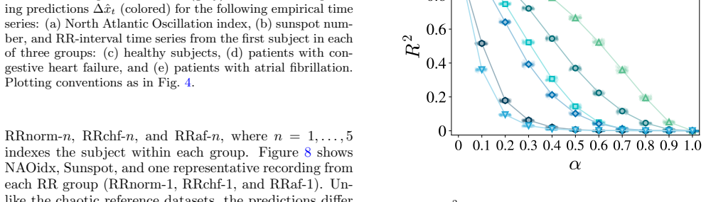
- The criterion tolerates finite levels of measurement noise: $R^2$ declines continuously with the noise-mixing coefficient $\alpha$, so the classification changes only when deterministic predictability is substantially destroyed.
- Short records of a few hundred samples usually suffice: synthetic chaos and noise are classified consistently at all tested lengths, and empirical records stabilize for $L_{\rm given} \ge 2000$.
- The score can serve as a continuous measure of how strongly observed dynamics support a deterministic description, not only as a binary label.
- The cross-prediction strategy can be transplanted to other recurrent neural network architectures, since only the readout is trained.
Reading between the lines
- A natural but untested extension is to apply the same scalar $R^2$ threshold to regime-switching or intermittently chaotic data, where the score would presumably interpolate between the deterministic and stochastic regimes.
- Because the reservoir implicitly builds an embedding, the method may be sensitive to sampling rate; the authors' observation that downsampling SGAMP improved $R^2$ suggests temporal resolution itself can shift the classification, which deserves systematic testing.
- The threshold 0.5 is operational rather than derived from first principles; the wide gap seen in synthetic data (near unity versus below 0.1) suggests a more conservative threshold could be more robust on mixed empirical records.
- A practical tool could combine the cross-prediction $R^2$ with surrogate-data tests: if phase-randomized or shuffled surrogates of the same series also exceed the threshold, the deterministic label would be suspect.
Editorial analysis
A structured set of objections, weighed in public.
Referee Report
Summary. The paper proposes a reservoir-computing cross-prediction scheme for distinguishing deterministic chaos from stochastic noise from scalar time series. An echo state network is trained to predict the first difference Δx_{t+1}=x_{t+2}-x_{t+1} from the current value x_t, and the squared Pearson correlation R² between true and predicted differences is proposed as a classifier: R²>0.5 is labeled chaos and R²<0.5 noise. The method is applied to seven synthetic chaotic systems, six synthetic noise processes, and several empirical datasets, with additional robustness experiments varying additive noise, time-series length, and prediction lag.
Significance. The cross-prediction idea is attractive: it combines short-term predictability with a deterministic-flow test, and the paper presents a broad, clearly described validation across synthetic and empirical data. The reservoir implementation is transparent and the pseudo-code in Algorithm 1 makes the procedure reproducible. The robustness analyses in Sec. IV (noise mixing, finite length, prediction lag) are a strength and give useful practical information. If the universal R²>0.5 threshold were valid, this would be a practical advance over embedding-based methods. However, the threshold is not universal: a simple AR(1) noise process violates it, and the reported R² values are inflated by per-dataset hyperparameter optimization and by selecting the top 100 of 200 reservoir realizations. The paper is better read as a promising heuristic with benchmark-specific separation than as a quantitative law.
major comments (3)
- [Sec. IIA, Eq. (3), Fig. 6] The proposed criterion R²>0.5 ⇒ chaos is violated by a stationary AR(1) process x_{t+1}=φx_t+ε_t with negative autocorrelation. The conditional expectation of Δx_{t+1}=x_{t+2}-x_{t+1} given x_t is φ(φ-1)x_t, and the squared Pearson correlation between Δx_{t+1} and this optimal predictor is R²=φ²(1-φ)/2. For φ=-0.8 this gives R²≈0.576>0.5, and for φ=-0.9 it gives ≈0.77. This is a purely stochastic, stationary linear process with no deterministic flow, so the theoretical optimum of the cross-prediction task exceeds the paper's chaos threshold. The noise set in Sec. IIIA and Fig. 6 contains no negatively autocorrelated process, so the observed separation does not establish the claimed generality. Since the reservoir state can represent x_t (e.g., in the linear regime of tanh) and the readout is linear, an ESN can in principle realize this optimal predictor; the paper's hyperparameter optimization and realization selection would only push R² upward. The abstract's statement that R² provides a quantitative criterion for distinguishing chaos from noise is therefore not supported as stated.
- [Sec. VI, Algorithm 1, lines 16-18] The reported R² is computed after choosing the best hyperparameters on each dataset using the same CV5 folds, and the final score is the mean over the top 100 of 200 reservoir realizations ranked by validation RMSE. Selecting realizations by validation RMSE is a form of peeking at the validation set; it biases R² upward, most strongly for noise processes where many realizations have near-zero skill and only a few appear predictive by chance. The threshold R²=0.5 is then chosen after observing the distributions in Figs. 6 and 9. Thus the 'quantitative criterion' is partly a post-hoc fitted decision boundary applied to an optimized score, not a fixed, parameter-free law. The authors should report R² without the top-100 selection, or use nested cross-validation, and should describe how the threshold was selected before seeing the data.
- [Sec. VIB, Tables IV-VI] All six reservoir hyperparameters are optimized separately for each dataset, prediction scheme, and lag on the same data subsequently used for evaluation, with no independent test set. Because the per-dataset optimization can exploit chance regularities in each realization, the reported R² values are not directly comparable across datasets, and the separation in Fig. 6 may be optimistically biased. To support a universal quantitative criterion, the authors should validate with a fixed or lightly tuned hyperparameter set, or with nested cross-validation that leaves untouched data for final evaluation. This is a load-bearing issue because the paper's main claim is a single threshold that holds across all datasets, not merely a demonstration that some tuning can separate benchmark examples.
minor comments (5)
- [Eq. (3)] The notation R² for the squared Pearson correlation is easily confused with the coefficient of determination; please add an explicit sentence distinguishing these quantities.
- [Sec. IIA] The statement that the 'restricted inductive bias' of a fixed reservoir and linear readout reduces memorization of stochastic fluctuations is an empirical assumption, not a theorem; the AR(1) counterexample in the major comments shows that this bias does not automatically exclude stochastic processes from high R².
- [Fig. 6] The synthetic noise set includes fBm, which is non-stationary, alongside stationary processes; the paper should state whether the proposed criterion is intended to apply to non-stationary noise, since fBm has different properties from the other noise benchmarks.
- [Table I] The final column '≥2000' summarizes the results for L_given=2000, 5000, and 10000, but the text does not specify whether the hyperparameters were re-optimized at each length; please clarify.
- [Appendix B] The optimized hyperparameter tables would be more useful if accompanied by the corresponding achieved R² values, so readers can see the variability across the 200 reservoir realizations rather than only the top-100 summary.
Circularity Check
No definitional circularity: R^2 is a genuinely out-of-sample cross-validation score, and the 0.5 threshold is an explicit operational rule rather than a derived or fitted parameter.
full rationale
The paper's central quantity, R^2, is computed on held-out validation folds after training the linear readout on the remaining folds, so it is not equal to a training objective by construction. The threshold 0.5 is introduced explicitly as an operational classification rule ('we operationally classify time series with R^2 > 0.5 as chaos and those with R^2 < 0.5 as noise'), not as a theorem derived from first principles. The fixed-reservoir/linear-readout restriction is stated as an architectural assumption, and the empirical separation between chaotic systems and noise processes is presented as a benchmark demonstration rather than as a mathematically forced consequence. The only self-citations in the paper (Refs. [61] and [62], both by the first author) appear in the introduction as background on reservoir computing recovering chaotic attractors under noise; they are not used as load-bearing justification for the chaos/noise criterion. The skeptical AR(1) counterexample is a potential false-positive limitation of the empirical generalization, but it does not show that the paper's R^2 values reduce to its inputs by construction. Hyperparameter optimization on the same datasets and top-100 realization selection may inflate reported R^2 values, but this is a statistical optimism concern, not a definitional circularity. No equation in the paper defines the criterion in terms of itself, and no fitted parameter is renamed as a prediction. Hence no significant circularity is present.
Assumptions & free parameters
free parameters (3)
- Classification threshold R^2 = 0.5 =
0.5
- Reservoir hyperparameters (n, rho, sigma_in, a_leak, beta, k) =
Varies per dataset; see Tables IV-VI
- Number of top reservoir realizations reported =
100 out of 200
assumptions (4)
- domain assumption The reservoir state provides a sufficient representation of the underlying dynamics from scalar input without explicit delay-coordinate embedding.
- domain assumption The fixed reservoir and linear readout impose a restricted inductive bias that reduces memorization of stochastic fluctuations.
- domain assumption The tested noise processes (Gaussian, uniform, Cauchy, flicker, fBm, fGn) are representative of 'noise' for the proposed criterion.
- standard math Standard ridge regression and Pearson correlation are appropriate tools for the prediction and scoring tasks.
Cite this review
Pith. "Pith review of Learning a quantitative criterion for distinguishing chaos from noise." pith.science (2026). https://pith.science/paper/GST64RZH
@misc{pith2026260807109,
  author       = {Pith},
  title        = {Pith review of: Learning a quantitative criterion for distinguishing chaos from noise},
  year         = {2026},
  howpublished = {\url{https://pith.science/paper/GST64RZH}},
  note         = {Machine review of arXiv:2608.07109}
}
read the original abstract
Distinguishing chaos from noise using time-series data is fundamentally challenging because both exhibit irregular fluctuations and share many statistical and dynamical characteristics. Existing methods face two key limitations: temporally correlated noise can yield spurious signatures of chaos, and analyses of scalar time series often require explicit choices of embedding parameters. Here, we propose a purely data-driven method for distinguishing chaos and noise based on a reservoir-computing framework with a cross-prediction scheme. In the proposed approach, the model is trained to predict the future change of a variable from its current value, thereby combining a short-term predictability test with a test of the smoothness of deterministic flows. The recurrent structure of reservoir computing enables effective prediction of high-dimensional chaotic dynamics even from scalar time series without explicit delay-coordinate reconstruction, while the cross-prediction framework strongly suppresses spurious predictive correlations arising from noise. We apply the proposed method to diverse synthetic and empirical time series. Chaotic systems consistently yield strong correlations between the true and predicted future changes, whereas noise processes remain clearly separated in a low-correlation regime. The method also exhibits substantial robustness to practical limitations in empirical data, including measurement noise, limited data length, and increasing prediction lag. These results demonstrate that the squared Pearson correlation coefficient provides a simple quantitative criterion for distinguishing chaos from noise directly from observed time-series data.
Figures


Figures from the paper (8 more)




Reference graph
Works this paper leans on
-
[1]
The syn- thetic chaotic datasets comprise both discrete-time and continuous-time systems
Synthetic chaotic systems All synthetic time series used in our analysis have a total length ofL given = 10,000 samples. The syn- thetic chaotic datasets comprise both discrete-time and continuous-time systems. Discrete-time systems are it- erated directly. Continuous-time systems are integrated numerically using a fourth-order Runge–Kutta method with a f...
-
[2]
•Gaussian noise (Gauss):An i.i.d
Synthetic noise processes We generate time series from the following noise pro- cesses with total lengthL given = 10,000 samples. •Gaussian noise (Gauss):An i.i.d. sequence drawn from the standard normal distribution,Xt ∼ N(0,1). •Uniform noise (Uniform):An i.i.d. sequence drawn from a uniform distribution on (0,1),X t ∼ U(0,1) with a flat probability den...
-
[3]
Unless otherwise stated below, the empirical datasets are analyzed at their full available lengths, with the normalization in Eq
Empirical datasets We evaluate the proposed method on a collection of empirical time series data spanning biomedical, physical, and geophysical systems. Unless otherwise stated below, the empirical datasets are analyzed at their full available lengths, with the normalization in Eq. (5) as the only preprocessing step. The specific time series lengthL given...
1937
-
[4]
Bradley and H
E. Bradley and H. Kantz, Chaos25, 097610 (2015)
2015
-
[5]
Kantz and T
H. Kantz and T. Schreiber,Nonlinear time series analysis (Cambridge university press, 2003)
2003
-
[6]
M. B. Kennel and S. Isabelle, Phys. Rev. A46, 3111 (1992)
1992
-
[7]
O. A. Rosso, H. Larrondo, M. T. Martin, A. Plastino, and M. A. Fuentes, Phys. Rev. Lett.99, 154102 (2007)
2007
-
[8]
D. J. Wales, Nature350, 485 (1991)
1991
Show all 93 references
-
[9]
Grassberger and I
P. Grassberger and I. Procaccia, Phys. Rev. Lett.50, 346 (1983)
1983
-
[10]
Grassberger and I
P. Grassberger and I. Procaccia, Physica D9, 189 (1983)
1983
-
[11]
A. Wolf, J. B. Swift, H. L. Swinney, and J. A. Vastano, Physica D16, 285 (1985)
1985
-
[12]
Theiler, Phys
J. Theiler, Phys. Lett. A155, 480 (1991)
1991
-
[13]
Grassberger and I
P. Grassberger and I. Procaccia, Phys. Rev. A28, 2591 (1983)
1983
-
[14]
Eckmann and D
J.-P. Eckmann and D. Ruelle, Physica D56, 185 (1992)
1992
-
[15]
A. R. Osborne and A. Provenzale, Physica D35, 357 (1989)
1989
-
[16]
Provenzale, A
A. Provenzale, A. R. Osborne, and R. Soj, Physica D47, 361 (1991)
1991
-
[17]
D¨ ammig and F
M. D¨ ammig and F. Mitschke, Phys. Lett. A178, 385 (1993)
1993
-
[18]
Tanaka, K
T. Tanaka, K. Aihara, and M. Taki, Phys. Rev. E54, 2122 (1996)
1996
-
[19]
Ikeguchi and K
T. Ikeguchi and K. Aihara, Int. J. Bifurcation Chaos7, 1267 (1997)
1997
-
[20]
Luque, L
B. Luque, L. Lacasa, F. J. Ballesteros, and A. Robledo, Chaos22, 013109 (2012)
2012
-
[21]
Barahona and C.-S
M. Barahona and C.-S. Poon, Nature381, 215 (1996)
1996
-
[22]
Lacasa and R
L. Lacasa and R. Toral, Phys. Rev. E82, 036120 (2010)
2010
-
[23]
Luque, L
B. Luque, L. Lacasa, F. J. Ballesteros, and A. Robledo, PLoS One6, e22411 (2011)
2011
-
[24]
Zhang and M
J. Zhang and M. Small, Phys. Rev. Lett.96, 238701 (2006)
2006
-
[25]
M. G. Ravetti, L. C. Carpi, B. A. Gon¸ calves, A. C. Frery, and O. A. Rosso, PLoS One9, e108004 (2014)
2014
-
[26]
Poon and M
C.-S. Poon and M. Barahona, Proc. Natl. Acad. Sci. U.S.A.98, 7107 (2001)
2001
-
[27]
Zhang, X
J. Zhang, X. Luo, and M. Small, Phys. Rev. E73, 016216 (2006)
2006
-
[28]
Zanin, Commun
M. Zanin, Commun. Nonlinear Sci. Numer. Simul.114, 106708 (2022)
2022
-
[29]
D. M. Wolpert and R. Miall, Proc. R. Soc. London, Ser. B242, 82 (1990)
1990
-
[30]
J. B. Borges, H. S. Ramos, R. A. Mini, O. A. Rosso, A. C. Frery, and A. A. Loureiro, Appl. Math. Comput. 362, 124554 (2019)
2019
-
[31]
Boaretto, R
B. Boaretto, R. C. Budzinski, K. L. Rossi, T. L. Prado, S. R. Lopes, and C. Masoller, Sci. Rep.11, 15789 (2021)
2021
-
[32]
Zunino, M
L. Zunino, M. C. Soriano, and O. A. Rosso, Phys. Rev. E86, 046210 (2012)
2012
-
[33]
T. L. Prado, B. R. R. Boaretto, G. Corso, G. Z. dos Santos Lima, J. Kurths, and S. R. Lopes, New J. Phys. 24, 033027 (2022)
2022
-
[34]
J. V. V. Flauzino, T. L. Prado, N. Marwan, J. Kurths, and S. R. Lopes, Phys. Rev. Lett.135, 097401 (2025)
2025
-
[35]
Olivares, A
F. Olivares, A. Plastino, and O. A. Rosso, Phys. Lett. A 376, 1577 (2012)
2012
-
[36]
J. M. Amig´ o, S. Zambrano, and M. A. Sanju´ an, EPL79, 50001 (2007)
2007
-
[37]
Quintero-Quiroz, S
C. Quintero-Quiroz, S. Pigolotti, M. Torrent, and C. Ma- soller, New J. Phys.17, 093002 (2015)
2015
-
[38]
Zanin and F
M. Zanin and F. Olivares, Commun. Phys.4, 190 (2021)
2021
-
[39]
J. M. Amig´ o, L. Kocarev, and J. Szczepanski, Phys. Lett. A355, 27 (2006)
2006
-
[40]
Kulp and L
C. Kulp and L. Zunino, Chaos24, 033116 (2014)
2014
-
[41]
J. M. Amig´ o, S. Zambrano, and M. A. Sanju´ an, EPL83, 60005 (2008)
2008
-
[42]
L. C. Carpi, P. M. Saco, and O. A. Rosso, Physica A 389, 2020 (2010)
2010
-
[43]
O. A. Rosso, L. C. Carpi, P. M. Saco, M. G. Ravetti, A. Plastino, and H. A. Larrondo, Physica A391, 42 (2012)
2012
-
[44]
Tsonis and J
A. Tsonis and J. Elsner, Nature358, 217 (1992)
1992
-
[45]
U. S. Freitas, C. Letellier, and L. A. Aguirre, Phys. Rev. E79, 035201 (2009)
2009
-
[46]
J. Gao, J. Hu, X. Mao, and W.-w. Tung, Chaos Solitons Fractals45, 213 (2012)
2012
-
[47]
Sugihara and R
G. Sugihara and R. M. May, Nature344, 734 (1990)
1990
-
[48]
L. W. Salvino and R. Cawley, Phys. Rev. Lett.73, 1091 (1994)
1994
-
[49]
D. T. Kaplan and L. Glass, Phys. Rev. Lett.68, 427 (1992)
1992
-
[50]
Wayland, D
R. Wayland, D. Bromley, D. Pickett, and A. Passamante, Phys. Rev. Lett.70, 580 (1993)
1993
-
[51]
D. T. Kaplan and L. Glass, Physica D64, 431 (1993)
1993
-
[52]
Takens, inDynamical Systems and Turbulence, War- wick 1980, Lecture Notes in Mathematics, Vol
F. Takens, inDynamical Systems and Turbulence, War- wick 1980, Lecture Notes in Mathematics, Vol. 898, edited by D. Rand and L.-S. Young (Springer, Berlin, Heidelberg, 1981) pp. 366–381
1980
-
[53]
G. J. Ortega and E. Louis, Phys. Rev. Lett.81, 4345 (1998)
1998
-
[54]
Ikeguchi and K
T. Ikeguchi and K. Aihara, Phys. Rev. E55, 2530 (1997)
1997
-
[55]
Jeong, M
J. Jeong, M. S. Kim, and S. Y. Kim, Phys. Rev. E60, 831 (1999)
1999
-
[56]
Z. Lu, B. R. Hunt, and E. Ott, Chaos28, 061104 (2018)
2018
-
[57]
Jaeger and H
H. Jaeger and H. Haas, Science304, 78 (2004)
2004
-
[58]
Pathak, Z
J. Pathak, Z. Lu, B. R. Hunt, M. Girvan, and E. Ott, Chaos27, 121102 (2017)
2017
-
[59]
Pathak, B
J. Pathak, B. Hunt, M. Girvan, Z. Lu, and E. Ott, Phys. Rev. Lett.120, 024102 (2018)
2018
-
[60]
Zhai, L.-W
Z.-M. Zhai, L.-W. Kong, and Y.-C. Lai, Phys. Rev. Res. 5, 033127 (2023)
2023
-
[61]
Z. Lu, J. Pathak, B. Hunt, M. Girvan, R. Brockett, and E. Ott, Chaos27, 041102 (2017)
2017
-
[62]
Margazoglou and L
G. Margazoglou and L. Magri, Nonlinear Dyn.111, 8799 (2023)
2023
-
[63]
H. Fan, J. Jiang, C. Zhang, X. Wang, and Y.-C. Lai, Phys. Rev. Res.2, 012080 (2020)
2020
-
[64]
Gantert, J
C. Gantert, J. Honerkamp, and J. Timmer, Biol. Cybern. 66, 479 (1992)
1992
-
[65]
Choi and P
J. Choi and P. Kim, Chaos35, 083136 (2025)
2025
-
[66]
Choi and P
J. Choi and P. Kim, Knowl.-Based Syst.330, 114574 (2025)
2025
-
[67]
Cazelles and R
B. Cazelles and R. Ferriere, Nature355, 25 (1992)
1992
-
[68]
Langarica and F
S. Langarica and F. N´ u˜ nez, Eng. Appl. Artif. Intell.120, 105838 (2023)
2023
-
[69]
SadeghiRazlighi, A
M. SadeghiRazlighi, A. H. Jafari, S. M. Firoozabadi, and G. A. Shahidi, Australas. Phys. Eng. Sci. Med.35, 25 (2012)
2012
-
[70]
Gao and W.-w
J. Gao and W.-w. Tung, Biol. Cybern.86, 263 (2002)
2002
-
[71]
Sarbaz and H
Y. Sarbaz and H. Pourakbari, Biomed. Signal Process. Control61, 102040 (2020). 18
2020
-
[72]
J. R. M. Hosking, Water Resour. Res.20, 1898 (1984)
1984
-
[73]
Y. Liu, Y. Zhou, K. Yang, and X. Wang, IEEE Internet Things J.10, 14285 (2023)
2023
-
[74]
M. L. Heltberg, S. Krishna, and M. H. Jensen, Nat. Com- mun.10, 71 (2019)
2019
-
[75]
Timmer and M
J. Timmer and M. K¨ onig, Astron. Astrophys.300, 707 (1995)
1995
-
[76]
Santa Fe time series competition, dataset a: Fluctuations in a far-infrared laser,https://www.comp-engine.org/ browse/category/real/physics/laser, (accessed June 2026)
2026
-
[77]
Cesari, G
U. Cesari, G. De Pietro, E. Marciano, C. Niri, G. San- nino, and L. Verde, Comput. Electr. Eng.68, 310 (2018)
2018
-
[78]
Herzel, D
H. Herzel, D. Berry, I. R. Titze, and I. Steinecke, Chaos 5, 30 (1995)
1995
-
[79]
Tao and J
C. Tao and J. J. Jiang, Phys. Rev. E77, 061922 (2008)
2008
-
[80]
A. Mees, K. Aihara, M. Adachi, K. Judd, T. Ikeguchi, and G. Matsumoto, Phys. Lett. A169, 41 (1992)
1992
-
[81]
H¨ ubner, N
U. H¨ ubner, N. B. Abraham, and C. O. Weiss, Physical Review A40, 6354 (1989)
1989
-
[82]
Paydarfar, D
D. Paydarfar, D. B. Forger, and J. R. Clay, J. Neuro- physiol.96, 3338 (2006)
2006
-
[83]
Aihara and G
K. Aihara and G. Matsumoto, inChaos, edited by A. V. Holden (Manchester University Press and Princeton Uni- versity Press, Manchester and Princeton, NJ, 1986)
1986
-
[84]
Timmer, S
J. Timmer, S. H¨ außler, M. Lauk, and C.-H. L¨ ucking, Chaos10, 278 (2000)
2000
-
[85]
T. L. Prado, V. S. Machado, G. Corso, G. Z. d. S. Lima, and S. R. Lopes, Parameter free determination of opti- mum time delay (2020), arXiv:2010.02951
2020 arXiv
-
[86]
L. O. Chua, J. Circuits Syst. Comput.4, 117 (1994)
1994
-
[87]
Tremor dataset,https://jeti.uni-freiburg.de/path_ tremor/readme, (accessed June 2026)
2026
-
[88]
Glass, Chaos19, 028501 (2009)
L. Glass, Chaos19, 028501 (2009)
2009
-
[89]
gov/products/precip/CWlink/pna/nao.shtml, accessed June 2026
NOAA climate prediction center: Daily North Atlantic Oscillation (NAO) index,https://www.cpc.ncep.noaa. gov/products/precip/CWlink/pna/nao.shtml, accessed June 2026
2026
-
[90]
Toker, F
D. Toker, F. T. Sommer, and M. D’Esposito, Commun. Biol.3, 11 (2020)
2020
-
[91]
SILSO world data center: Sunspot number archive, http://www.sidc.be/silso/infosndtot, (accessed June 2026)
2026
-
[93]
PhysioNet chaos challenge: Is the normal heart rate chaotic?,https://archive.physionet.org/challenge/ chaos/, (accessed June 2026)
2026
-
[1950]
•Sunspot number (Sunspot):We use the daily total sunspot number (V2.0) from the Sunspot In- dex and Long-term Solar Observations (SILSO) repository [87]
A previous study reported a stochastic origin for these data [86]. •Sunspot number (Sunspot):We use the daily total sunspot number (V2.0) from the Sunspot In- dex and Long-term Solar Observations (SILSO) repository [87]. To avoid missing values in the early records, we use the...
1970
Reviewed August 10, 2026 · model on record in the stance chip above.
Discussion (0). Continue with ORCID to comment.