REVIEW 3 major objections 4 minor 43 references
A unifying framework for quantum algorithms for time-dependent non-unitary dynamics
T0 review · 3 major / 4 minor · reviewed 2026-08-10 · deepseek-v4-flash
Pith's one-line read This paper shows that time-dependent non-unitary linear dynamics can be autonomized with a clock variable into a time-independent linear system, and that combining it with Schrödingerization yields precision dependence log^{5/4}(1/ε)…
desk verdict The autonomization framework is clean and likely correct, but the advertised log^{5/4}(1/ε) precision dependence is not established: Lemma 2.1 omits the B(s)-derivatives that control the clock-direction regularity, so the main complexity claim is unsupported. read the letter →
The pith
A machine-rendered reading of the paper's core claim, the machinery that carries it, and where it could break.
The reading
What carries the argument
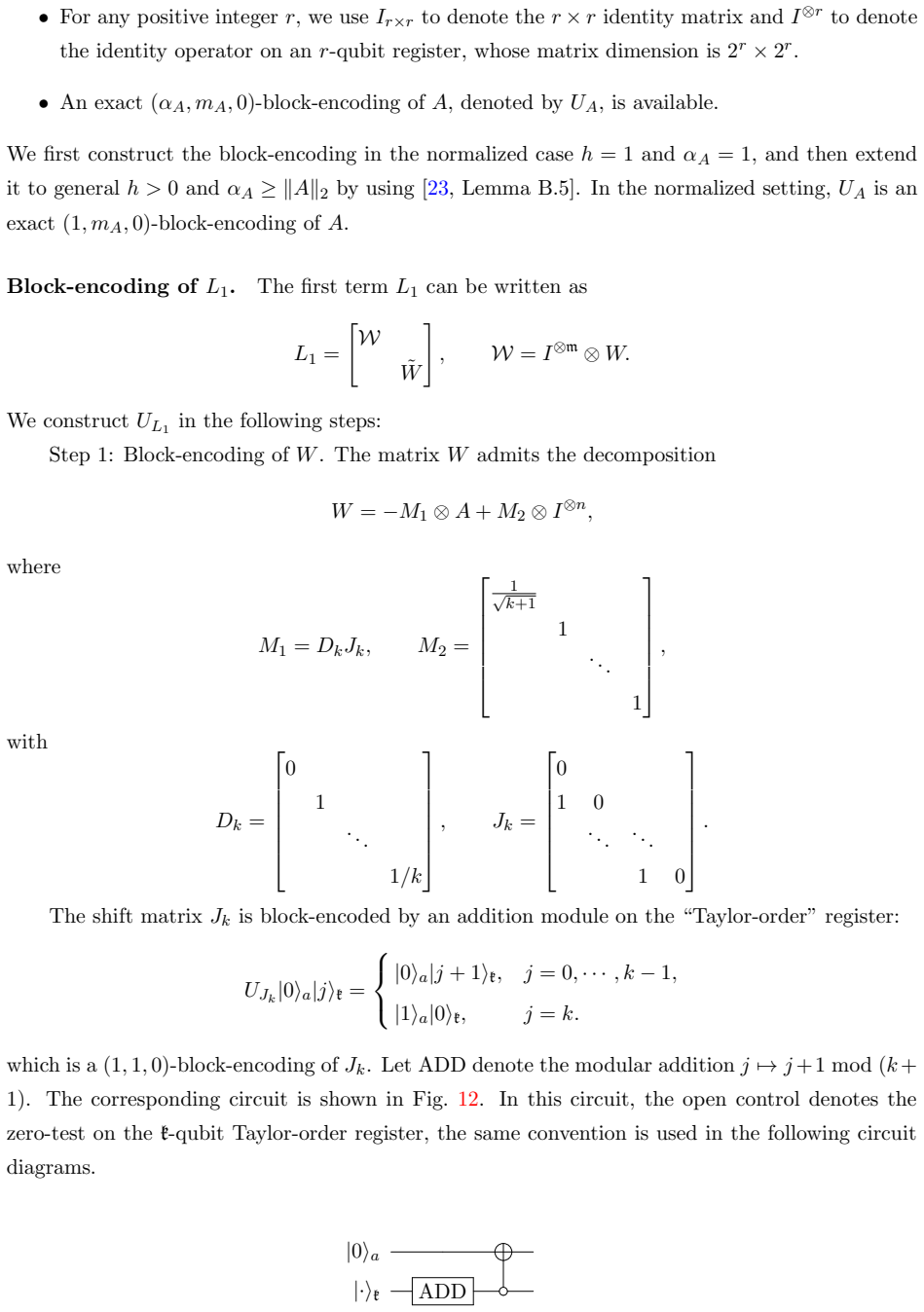
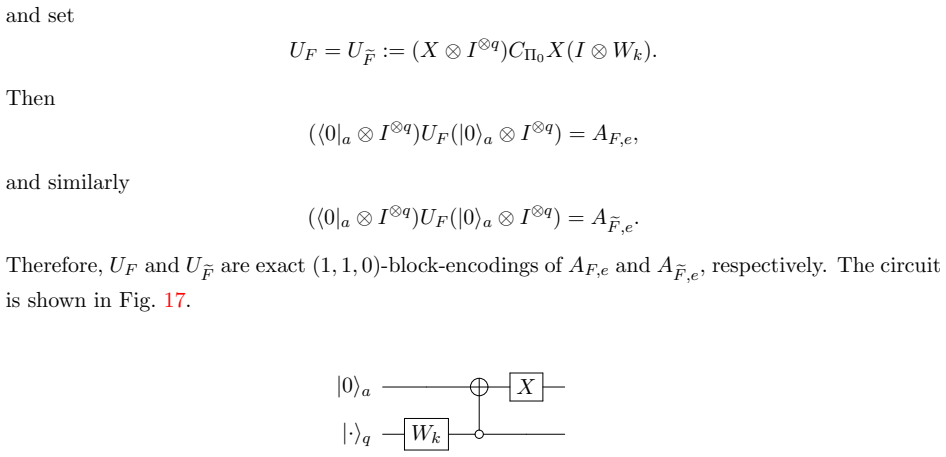
The carrying object is the clock-variable autonomization identity together with its Fourier spectral discretization. The paper adds a clock register $s$, freezes the coefficient matrix as $B(s)$, and solves a convection equation whose method-of-characteristics solution reproduces the original propagator; a smooth initial profile $G(s)$ with $G(0)=1$ that decays super-exponentially (one of $G_m$, $G_w$, $G_f$) makes the problem effectively periodic and controls the largest Fourier mode as $\mu_{s,\max} = O(\log^\beta(1/\delta_s))$ with $\beta=3,1,1/2$ respectively. This produces the explicit time-independent matrix $\bar{A}$, its block-encoding, and the recovery map $x_h(T) = R_x w(T)$ projected at the midpoint $s=T$. The same matrix is then shifted by $\gamma = 1/(2T)$ to restore dissipativity for Schrödingerization, or fed directly into the BCOW linear-system construction.
What would settle it
Take an exactly solvable non-autonomous system whose coefficients are only $C^k$ rather than analytic, run the autonomization construction for a decreasing sequence of targets $\delta_s$, and measure the largest Fourier mode $\mu_{s,\max}$ needed to keep $\|G - P_h G\|_{L^\infty} \le \delta_s$; if $\mu_{s,\max}$ grows like $\delta_s^{-1/(k-1/2)}$ rather than $O(\log^\beta(1/\delta_s))$, that polynomial blow-up would falsify the $\log^{5/4}(1/\varepsilon)$ complexity for that regularity class.
Extended reading notes
Core claim
The central claim is that the time-ordered exponential is not an obstacle for time-dependent non-unitary systems. For the enlarged homogeneous system $du/dt = B(t)u$, define $z$ by $\partial_t z + \partial_s z = B(s)z$, $z(0,s)=G(s)u(0)$, with $G(0)=1$; then $z(t,s=t)=G(0)u(t)$, exactly. Fourier-spectral discretization in $s$ converts this into a static matrix $\bar{A} = -iP_s \otimes I + \sum_l |l\rangle\langle l| \otimes B(s_l)$, which the paper block-encodes from HAM-T oracles for $A(s)$ and $F(s)$ plus a Fourier-differentiation gadget. The paper proves two instantiations: with Schrödingerization, $O(g_A \alpha_A T \log^{\max\{1+\beta/2, 3\beta/2\}}(g_A/\varepsilon))$ queries to the matrix oracles, which becomes $\log^{5/4}(1/\varepsilon)$ for the super-exponentially decaying profile $G_f$ ($\beta=1/2$); with a Taylor-expansion BCOW solver, $O(C_A^2 g_A \alpha_A T \log^{3(\beta+1)/2}(\alpha_A T C_A^2 g_A/\varepsilon))$ queries, and the analysis removes the diagonalizability assumption by bounding complexity through the growth factor $C(A) = \sup_t \|e^{At}\|$.
Load-bearing premise
The load-bearing assumption is that $A(t)$ and $b(t)$ are real analytic in time, because only then does the Fourier spectral error in the clock variable decay fast enough to keep the number of grid points logarithmic in the required accuracy; with merely finitely smooth coefficients the mesh size would grow polynomially and the $\log^{5/4}(1/\varepsilon)$ dependence is not established.
Editorial extensions
If this is right
- Any existing quantum ODE solver for time-independent non-unitary systems can be reused for time-dependent problems by consuming the autonomization matrix $\bar{A}$ and its block-encoding; time dependence is fully pushed into the HAM-T oracles.
- For the analytic clock profile $G_f$, the Schrödingerization combination uses $O(g_A \alpha_A T \log^{5/4}(g_A/\varepsilon))$ queries to the matrix oracles, improving the $\varepsilon$-dependence of earlier constructions.
- The BCOW combination inherits the same framework and its new analysis extends the algorithm to non-diagonalizable matrices, with cost controlled by the growth factor $C(A)$ instead of an eigenvector condition number.
- The recovery postselects on the single grid point $s=T$ and then the $x$-block; with amplitude amplification the success probability is $\Omega(1)$, so the algorithm outputs a state $\varepsilon$-close to $|x(T)\rangle$ with a success flag.
Reading between the lines
- A testable extension the paper leaves implicit: for coefficients that are only $C^k$ in time, the Fourier mesh would need to scale polynomially in $1/\delta_s$, so the $\log^{5/4}$ precision dependence is tied to analyticity; one could quantify the crossover by mollifying a $C^k$ coefficient and balancing regularization error against discretization error.
- The modular structure suggests a menu of clock profiles: the $\beta=1/2$ profile is optimal for the Schrödingerization query count, while a compactly supported profile ($\beta=3$) gives simpler boundary handling and might be preferable in implementations where exact support matters.
- The midpoint recovery condition ($s=T$ on an even grid) is a small numerical-engineering constraint that may generalize to other spectral discretizations, effectively giving a quantum method of characteristics for non-autonomous equations.
Editorial analysis
A structured set of objections, weighed in public.
Referee Report
Summary. The paper proposes an 'autonomization' framework for quantum simulation of time-dependent non-unitary linear ODEs. The non-autonomous system (1.1) is lifted via the clock-variable construction of Cao–Jin–Liu to an autonomous transport-type PDE (2.2), whose Fourier spectral discretization yields the explicit time-independent matrix Ā in (2.15). The framework is modular: Ā can be fed into any quantum ODE solver for time-independent systems. The authors combine Ā with the Schrödingerization method and with the BCOW Taylor-expansion solver, deriving query complexities in Theorems 3.1 and 4.2. The headline claim is that, under real-analyticity and dissipativity of A(t), the precision dependence of the Schrödingerization-based combination scales as log^{5/4}(1/ε), improving on the log^2(1/ε) scaling of existing approaches. Numerical experiments on a two-cavity system validate recovery of the target trajectory for both combinations.
Significance. The modular autonomization idea is attractive: it decouples the treatment of time dependence from the choice of the underlying time-independent solver, and the block-encoding circuits in Section 2.3 are explicit. The non-diagonalizable BCOW analysis in Section 4.2 is a useful extension of the original Berry–Childs–Ostrander–Wang result. If the complexity claims were fully established, the log^{5/4}(1/ε) precision dependence would be a noteworthy improvement over the competing log^2(1/ε) scaling. However, the two load-bearing analytical steps — the spectral error bound in Lemma 2.1 and the treatment of the clock-interval length in Theorem 3.1 — are not justified under the stated assumptions. The advertised precision dependence is therefore not currently established, although the framework and numerics remain plausible and potentially salvageable with strengthened assumptions and a corrected proof.
major comments (3)
- [Lemma 2.1, Section 2.2] The proof of Lemma 2.1 is not provided; it is asserted by 'following the similar arguments in [30]'. This does not transfer to the present setting. The exact solution (2.5) is z(T,s) = Texp(∫_0^T B(s-T+τ)dτ)G(s-T)u_0, so ∂_s^r z(T,·) involves derivatives of B(s) of orders up to r, not just derivatives of G. The Fourier projection error (2.18) controls the error only through the regularity of the function being projected, which is z(T,·), not G alone. Consequently the bound ∥z(T,s_l) - z_h(T,s_l)∥ ≲ (Δs)^{r-1/2}∥G^{(r)}∥_{L^2(I_s)}∥u(0)∥ in Lemma 2.1 is not established. The assumption after (2.1) that A,b are real analytic on R does not supply uniform control of the relevant derivatives on the interval I_s, whose length grows with δ_s^{-1} for the profile G_f. A concrete counterexample to the claimed bound is A(t)=i e^t I with b=0, for which z(T,s) = exp(i(e^s - e^{s-T}))G(s-T)u_0; the r-th s-derivative grows like e^{rs} on I_s, so the spectral error is not governed by ∥G^{(r)}∥ alone. The proof must either estimate the full r-th derivative of z(T,·), including the B-dependent terms, or impose explicit regularity and boundedness assumptions on B(s) over I_s.
- [Assumptions after (2.1) and Theorem 3.1] The advertised log^{5/4}(1/ε) precision dependence is not derived under the stated assumptions. The interval I_s = [-R_s, R_s+2T] has R_s = 2 log^{1/2}(1/δ_s) for the headline profile G_f in (2.9), so the grid points s_l range over an interval whose length grows with ε^{-1}. The quantity α_A in (2.22) is defined as max_{0≤l≤N_s-1}∥A(s_l)∥ and enters the final bound O(g_A α_A T log^{max{1+β/2,3β/2}}(g_A/ε)) in Theorem 3.1. Real analyticity on R does not prevent α_A from growing on this expanding interval. For the dissipative, real-analytic example A(t)=i e^t I, one has α_A = e^{R_s+2T} = e^{O(log^{1/2}(1/δ_s))}, which converts the stated complexity into e^{O(log^{1/2}(1/ε))} instead of log^{5/4}(1/ε). The paper needs either a uniform boundedness assumption on A(s) and b(s) (and suitable derivatives) over I_s with a constant independent of ε, or a more careful statement that separates the ε-dependence of α_A from the precision dependence. As written, the abstract's 'precision dependence can scale as log^{5/4}(1/ε)' is not supported.
- [Equation (2.6), Section 2.1] The definition of G_m is inconsistent with the stated property G_m(0)=1. With η(s)=e^{1/(s^2-1)} for |s|<1, one has η(0)=e^{-1}, hence G_m(0)=e^{e^{-1}}≠1. If the intended mollifier is η(s)=1/(s^2-1), then G_m(0)=e^{-1}≠1. The manuscript uses G(0)=1 in the recovery map (2.17), in the success-probability computation in Theorem 3.1 step (2), and in Theorem 4.2. This is a concrete error in a central definition. The profile should be normalized by dividing by G_m(0), or η should be shifted so that η(0)=0; the derivative estimates in Theorem 2.2 are unaffected up to constants, but the text and recovery formulas must be corrected.
minor comments (4)
- [Remark 3.2 and Introduction] The claimed improvement over [26] is stated without giving the comparison complexity of [26]. To make the 'improving upon log^2(1/ε)' assertion verifiable, the authors should state the query complexity of [26] in the same notation and identify precisely the source of the saving.
- [Lemma 2.1 proof] In the proof of Lemma 2.1, the phrase '∀l≥0' is unclear because the grid index l ranges over 0≤l≤N_s-1 and the pointwise estimate is needed at the recovery point s=T=s_{N_s/2}; this should be stated directly.
- [Section 2.2, Eq. (2.18)] The pointwise Fourier projection estimate from [34] applies to periodic functions; for the profiles G_w and G_f, which are only approximately supported, the boundary values of G and its derivatives at s=±R_s are small but not exactly zero. The additional contribution of the boundary discontinuity to the estimate (2.18) should be addressed explicitly rather than left to the cited literature.
- [Acknowledgements] The acknowledgements mention 'NL acknowledges funding from ...', but the author list contains no 'NL'. This appears to be a leftover from a different version and should be corrected (or the name spelled out) before publication.
Circularity Check
No significant circularity: the derivation is an analytic reduction with explicit error estimates, and prior-work citations are used as external building blocks rather than as definitions of the target result.
full rationale
The paper's central chain is a mathematical derivation, not a fit. The enlarged system (2.1) is constructed so that F(t)r(t)=b(t) by the definitions of F and r, and Theorem 2.1 proves z(T,T)=G(0)u(T) by a direct characteristic calculation; the recovery map is then defined to extract u(T), so there is no fitted parameter being renamed as a prediction. The profile choices G_m, G_w, and G_f are explicit functions with stated estimates; the parameter a and the shift gamma are chosen to satisfy error and dissipativity bounds, not to reproduce the claimed complexity. The self-citations to [1] and [30] supply the clock-variable construction, the smooth-profile derivative estimates, and the Schroedingerization complexity lemma. These are prior published results whose stated assumptions do not include the present autonomization claim or the log^{5/4}(1/epsilon) precision target, so under the reviewing rules they count as independent support rather than circularity. The paper's possible correctness gap, namely that Lemma 2.1 bounds the Fourier error only through G^(r) and omits derivatives of B(s), and the fact that alpha_A may carry epsilon-dependence for real-analytic but unbounded coefficients, is a mathematical soundness concern, not a circularity: the claimed bound does not reduce by construction to an input or to a self-citation. The numerical experiments are benchmarked against a reference solution and do not feed fitted values back into the theorem. No step of the derivation is equivalent to its own inputs by definition, and no fitted parameter is relabeled as a prediction.
Assumptions & free parameters
free parameters (2)
- shift γ =
1/(2T)
- profile scale a for G_w =
2 log^{1/2}(1/δ_s)
assumptions (7)
- domain assumption A(t)+A†(t) ⪯ O for t ∈ [0,T]
- domain assumption A(t) and b(t) are real analytic on R
- domain assumption Exact HAM-T block-encodings of A(s_l) and F(s_l) are available for all grid points
- ad hoc to paper G(s) can be chosen with G(0)=1 and (near-)compact support to impose periodic boundary conditions
- standard math Standard pointwise Fourier projection error estimate (2.18)
- standard math Smooth-initialization and profile estimates from [30]
- standard math QSVT-based Hamiltonian simulation of time-independent H is available
Cite this review
Pith. "Pith review of A unifying framework for quantum algorithms for time-dependent non-unitary dynamics." pith.science (2026). https://pith.science/paper/FPCQABBW
@misc{pith2026260807133,
  author       = {Pith},
  title        = {Pith review of: A unifying framework for quantum algorithms for time-dependent non-unitary dynamics},
  year         = {2026},
  howpublished = {\url{https://pith.science/paper/FPCQABBW}},
  note         = {Machine review of arXiv:2608.07133}
}
abstract
Quantum algorithms for simulating linear differential equations have attracted growing interest, driven by applications ranging from Hamiltonian dynamics to general non-unitary dynamics. While time-independent cases are well studied, time-dependent non-unitary dynamics remains considerably less explored, and it is unclear how to systematically adapt existing solvers for time-independent systems to such problems. In this work, we address this gap by introducing an autonomization framework based on the clock-variable formulation, a technique originally developed for time-dependent Hamiltonian systems in~\cite{CJL23TimeSchr}. By lifting the original non-autonomous system to an autonomous transport-type equation on an extended space and applying the Fourier spectral discretization in the clock variable, we obtain an explicit time-independent linear system, together with a suitable initial state and a recovery map for the target solution. Crucially, this formulation decouples the treatment of time dependence from the choice of the quantum ODE solver, thereby enabling the direct application of existing solvers designed for time-independent systems to the resulting autonomous problem. We combine this framework with Schr\"odingerization and a Taylor-expansion-based quantum ODE solver. In the Schr\"odingerization-based combination, our complexity analysis shows that the precision dependence can scale as $\log^{5/4}(1/\varepsilon)$, improving upon the $\log^2(1/\varepsilon)$ scaling found in existing approaches. Numerical experiments validate the autonomization formulation and confirm the successful recovery of the target solution.
Figures


Figures from the paper (16 more)






Reference graph
Works this paper leans on
-
[1]
Y. Cao, S. Jin, and N. Liu. Quantum simulation for time-dependent Hamiltonians – with applications to non-autonomous ordinary and partial differential equations.Journal of Physics A: Mathematical and Theoretical, 58(15):155304, 2025
work page 2025
-
[30]
S. Jin, N. Liu, C. Ma, Y. Peng, and Y. Yu. On the Schr¨ odingerization method for linear non-unitary dynamics with optimal dependence on matrix queries.Commun. Math. Sci., 24(2):565–592, 2026
2026
-
[2]
D. W. Berry, A. M. Childs, and R. Kothari. Hamiltonian simulation with nearly optimal dependence on all parameters. In2015 IEEE 56th Annual Symposium on Foundations of Computer Science, pages 792–809, 2015
work page 2015
-
[3]
G. H. Low and N. Wiebe. Hamiltonian simulation in the interaction picture. arXiv:1805.00675v2, 2019. 28
arXiv 2019
-
[4]
D. W. Berry, A. M. Childs, Y. Su, X. Wang, and N. Wiebe. Time-dependent Hamiltonian simulation withL 1-norm scaling.Quantum, 4:254, 2020
work page 2020
-
[5]
Y. Cao, A. Papageorgiou, I. Petras, J. Traub, and S. Kais. Quantum algorithm and circuit design solving the Poisson equation.New J. Phys., 15:013021, 2013
work page 2013
-
[6]
D. W. Berry. High-order quantum algorithm for solving linear differential equations.J. Phys. A: Math. Theor., 47(10):105301, 17 pp., 2014
work page 2014
-
[7]
A. Montanaro and S. Pallister. Quantum algorithms and the finite element method.Phys. Rev. A, 93:032324, 14 pp., 2016
work page 2016
Show all 43 references
-
[8]
P. C. S. Costa, S. Jordan, and A. Ostrander. Quantum algorithm for simulating the wave equation.Phys. Rev. A, 99:012323, 22 pp., 2019
2019
-
[9]
Engel, G
A. Engel, G. Smith, and S. E. Parker. Quantum algorithm for the Vlasov equation.Phys. Rev. A, 100:062315, Dec 2019
2019
-
[10]
A. W. Childs and J. Liu. Quantum spectral methods for differential equations.Comm. Math. Phys., 375(2):1427–1457, 2020
2020
-
[11]
Linden, A
N. Linden, A. Montanaro, and C. Shao. Quantum vs. classical algorithms for solving the heat equation.Commun. Math. Phys., 395(2):601–641, 2022
2022
-
[12]
A. M. Childs, J. P. Liu, and A. Ostrander. High-precision quantum algorithms for partial differential equations.Quantum, 5:574, 2021
2021
-
[13]
S. Jin, N. Liu, and Y. Yu. Time complexity analysis of quantum difference methods for linear high dimensional and multiscale partial differential equations.J. Comput. Phys., 471:111641, 2022
2022
-
[14]
S. Jin, N. Liu, and Y. Yu. Time complexity analysis of quantum algorithms via linear represen- tations for nonlinear ordinary and partial differential equations.J. Comput. Phys., 487:112149, 2023
2023
-
[15]
S. Jin, X. Li, N. Liu, and Y. Yu. Quantum simulation for quantum dynamics with artificial boundary conditions.SIAM J. Sci. Comput., 46:B403–B421, 2024
2024
-
[16]
S. Jin, N. Liu, and Y. Yu. Quantum simulation of partial differential equations: Applications and detailed analysis.Phys. Rev. A, 108:032603, 2023
2023
-
[17]
S. Jin, N. Liu, and Y. Yu. Quantum simulation of partial differential equations via Schr¨ odingerisation.arXiv:2212.13969, 2022
2022 arXiv
-
[18]
S. Jin, X. Li, N. Liu, and Y. Yu. Quantum simulation for partial differential equations with physical boundary or interface conditions.J. Comp. Phys., 498:112707, 2024
2024
-
[19]
Jin and N
S. Jin and N. Liu. Quantum algorithms for nonlinear partial differential equations.Bull. Sci. math, 194:103457, 2024. 29
2024
-
[20]
D. W. Berry, A. M. Childs, A. Ostrander, and G. Wang. Quantum algorithm for linear differential equations with exponentially improved dependence on precision.Comm. Math. Phys., 356(3):1057–1081, 2017
2017
-
[21]
H. C. Wu and X. Li. Structure-preserving quantum algorithms for linear and nonlinear Hamil- tonian systems.arXiv:2411.03599, 2024
2024 arXiv
-
[22]
H. Krovi. Improved quantum algorithms for linear and nonlinear differential equations.Quan- tum, 7:913, 2023
2023
-
[23]
D. Dong, Y. Li, and J. Xue. A quantum algorithm for linear autonomous differential equations via Pad´ e approximation.Quantum, 9:1770, 2025
2025
-
[24]
D. An, J. Liu, and L. Lin. Linear combination of Hamiltonian simulation for non-unitary dynamics with optimal state preparation cost.Phys. Rev. Lett., 131(15):150603, 2023
2023
-
[25]
D. An, A. M. Childs, and L. Lin. Quantum algorithm for linear non-unitary dynamics with near-optimal dependence on all parameters.Commun. Math. Phys., 407(1):19, 2026
2026
-
[26]
G. H. Low and R. D. Somma. Optimal quantum simulation of linear non-unitary dynamics. arXiv:2508.19238, 2025
2025 arXiv
-
[27]
Wang, H.-Y
C. Wang, H.-Y. Liu, C. Xue, X.-N. Zhuang, M. Dou, Z.-Y. Chen, and G.-P. Guo. Quan- tum simulation of non-Hermitian special functions and dynamics via contour-based matrix decomposition.Quantum Sci. Technol., 11(3):035027, 2026
2026
-
[28]
S. Jin, C. Ma, and E. Zuazua. Transmutation-based quantum simulation for non-unitary dynamics.arXiv:2601.03616, 2026
2026 arXiv
-
[29]
S. Jin, N. Liu, and C. Ma. On Schr¨ odingerization-based quantum algorithms for linear dy- namical systems with inhomogeneous terms.SIAM J. Numer. Anal., 63(4):1861–1885, 2025
2025
-
[31]
X. Li. From linear differential equations to unitaries: a moment-matching dilation framework with near-optimal quantum algorithms.arXiv:2507.10285, 2025
2025
-
[32]
D. W. Berry and P. C. S. Costa. Quantum algorithm for time-dependent differential equations using Dyson series.Quantum, 8:1369, 2024
2024
-
[33]
D. Fang, L. Lin, and Y. Tong. Time-marching based quantum solvers for time-dependent linear differential equations.Quantum, 7:955, 2023
2023
-
[34]
J. Shen, T. Tang, and L. Wang.Spectral methods: algorithms, analysis and applications. Springer Science & Business Media, 2011. 30
2011
-
[35]
Gily´ en, Y
A. Gily´ en, Y. Su, G. Low, and N. Wiebe. Quantum singular value transformation and be- yond: exponential improvements for quantum matrix arithmetics.arXiv:1806.01838, page arXiv:1806.01838, 2018
2018 arXiv
-
[36]
Gily´ en, Y
A. Gily´ en, Y. Su, G. Low, and N. Wiebe. Quantum singular value transformation and beyond: exponential improvements for quantum matrix arithmetics. InProceedings of the 51st Annual ACM SIGACT Symposium on Theory of Computing, pages 193–204. STOC, 2019
2019
-
[37]
Chakraborty, A
S. Chakraborty, A. Gily´ en, and S. Jeffery. The power of block-encoded matrix powers: im- proved regression techniques via faster Hamiltonian simulation. In46th International Collo- quium on Automata, Languages, and Programming (ICALP 2019), pages 33:1–33:14. ICALP, 2019
2019
-
[38]
L. Lin. Lecture notes on quantum algorithms for scientific computation.arXiv:2201.08309, 2022
2022 arXiv
-
[39]
A. Mock. Time-modulated coupled-cavity system for optical switching.The Applied Compu- tational Electromagnetics Society Journal, 35(11):1443–1444, 2020
2020
-
[40]
W. Suh, Z. Wang, and S. Fan. Temporal coupled-mode theory and the presence of non- orthogonal modes in lossless multimode cavities.IEEE Journal of Quantum Electronics, 40(10):1511–1518, 2004
2004
-
[41]
D. An, J. Liu, D. Wang, and Q. Zhao. Quantum differential equation solvers: limitations and fast-forwarding.Commun. Math. Phys., 406(8):189, 2025
2025
-
[42]
M¨ ott¨ onen, J
M. M¨ ott¨ onen, J. J. Vartiainen, V. Bergholm, and M. M. Salomaa. Quantum circuits for general multiqubit gates.Phys. Rev. Lett., 93:130502, 2004
2004
-
[43]
Taylor-order
D. Camps and R. Van Beeumen. F ABLE: fast approximate quantum circuits for block- encodings. In2022 IEEE International Conference on Quantum Computing and Engineering (QCE), pages 104–113. IEEE, 2022. A New complexity bound for the BCOW algorithm A.1 Solution error Letx i,h =x...
2022
Reviewed August 10, 2026 · model on record in the stance chip above.
Discussion (0). Continue with ORCID to comment.