A transient nonlinear finite element framework and implementation of coupled electro-chemo-mechanics of polyelectrolyte hydrogels

Bibekananda Datta; Brandon K. Zimmerman; Thao D. Nguyen

REVIEW 2 major objections 5 minor 18 references

A transient nonlinear finite element framework and implementation of coupled electro-chemo-mechanics of polyelectrolyte hydrogels

T0 review · 2 major / 5 minor · reviewed 2026-08-11 · deepseek-v4-flash

Challenge this review Re-run · record.json Download PDF Read on arXiv ↗ Review JSON

Pith's one-line read A monolithic finite element framework couples large-deformation mechanics, solvent transport, and ion diffusion to simulate polyelectrolyte hydrogels across swelling, consolidation, and bending.

desk verdict The framework and the open-source UEL implementation are solid and genuinely useful, but the validation is partly a fit with an unphysically large solvent diffusivity, so the abstract's 'validated' claim is too strong. read the letter →

arxiv 2608.07638 v1 pith:JD3LPJWW submitted 2026-08-07 cond-mat.soft

Bibekananda Datta , Brandon K. Zimmerman , Thao D. Nguyen This is my paper · ORCID

classification cond-mat.soft

keywords polyelectrolytehydrogelsfiniteelementanalysiselectro-chemo-mechanicstransientswellingDonnanpotentialhydrogelbilayeractuatorconsolidation

verification ladder T0 review T1 audit T2 compute T3 formal

The pith

A machine-rendered reading of the paper's core claim, the machinery that carries it, and where it could break.

The reading

The paper claims that the fully coupled electro-chemo-mechanical response of polyelectrolyte hydrogels—large swelling, ion exchange, consolidation under load, and bending—can be computed with a single monolithic finite element framework. It implements the theory as a user element in a standard commercial finite element solver, treating the gel as locally electroneutral so the electric potential is solved at each integration point rather than as a global field. The implementation is validated against transient free-swelling experiments of a cationic DMAEA gel in salt solutions of varying ionic strength, then applied to a gel-elastomer bilayer actuator and confined compression. If the approach holds, designers of hydrogel actuators, sensors, and cartilage-like load-bearing materials have a reusable computational tool that captures the interplay of deformation, solvent transport, and ion diffusion in one simulation.

What carries the argument

The load-bearing mechanism is a monolithic, Total Lagrangian, semi-discrete Galerkin formulation with nodal degrees of freedom $(\mathbf{u}, \mu_w, \omega_{\beta_k})$: displacement, solvent chemical potential, and each ion's electrochemical potential. At every Gauss point a local Newton iteration solves the constitutive residuals for the solvent chemical potential, the ion electrochemical potentials, and the electroneutrality constraint, yielding the internal variables $(C_w, C_{\beta_k}, \psi)$; consistent tangents then follow from the implicit function theorem applied to that local system. Volumetric locking from near-incompressibility is mitigated with the F-bar modification, in which the volumetric part of the deformation gradient is evaluated at the element centroid. This local-solve architecture is what lets a single user element carry the full coupling without a global electric-potential field.

What would settle it

A direct test would measure time-resolved solvent and ion concentration profiles inside a swelling gel without fitting the transport coefficients to the same swelling curve—for example, by tracking water-content fronts with MRI or fluorescence and comparing the speed of the front and the sign-change time in a bilayer actuator to model predictions made with independently measured mobilities.

Watch

Extended reading notes

Core claim

The paper's central claim is that fully coupled transient electro-chemo-mechanics of a polyelectrolyte gel can be reduced to a single monolithic finite element problem whose unknowns are the displacement, the solvent chemical potential, and the electrochemical potentials of the mobile ions, with the electric potential determined locally. The gel is treated as an electroneutral medium, so instead of solving Maxwell's equation the code enforces $z_{\rm fix}C_{\rm fix} + \sum_{\beta_k} z_{\beta_k} C_{\beta_k} = 0$ at every integration point; the potential $\psi$ plays the role of a local Lagrange multiplier, giving the Donnan potential. On this basis the paper derives a Total Lagrangian weak form, backward-Euler time discretization, a local Newton solve for concentrations and potential, and consistent tangent stiffness matrices, and packages the result as a user element. Validation against transient free-swelling experiments of a cationic DMAEA gel in NaCl baths of different ionic strengths supports the claim that the framework captures the driving physics; the same framework is then used to predict the transient curvature reversal of a gel-elastomer bilayer and the exudation-driven consolidation of a confined gel under compression.

Load-bearing premise

The load-bearing premise is that the transient behavior can be represented by a simple Fickian diffusion law with a single constant effective solvent diffusion coefficient, even though matching the swelling data required a value roughly 450 times the self-diffusion coefficient of water.

Editorial extensions

If this is right

The same calibrated model reproduces the two-cycle deswelling–swelling response of a cationic gel as the bath ionic strength alternates between 0.05 M and 0.2 M, so cyclic salt-stimulus behavior is accessible to simulation.
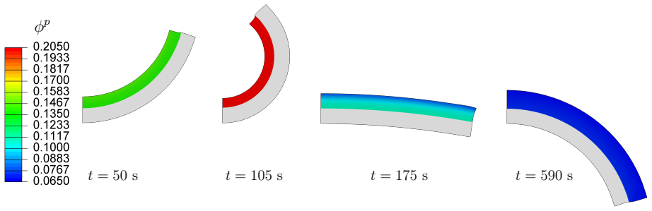
For gel-elastomer bilayers, the model predicts a sign reversal in curvature: water leaves first and bends the structure one way, then slower ion uptake drags water back and bends it the other way; design of salt-driven actuators must account for this transient.
Under confined compression, the model shows that solvent and ion exudation through a free-draining boundary is what relaxes compressive stress, with the equilibrium consolidation strain set by how swollen, and therefore how soft, the gel was before loading.
Parametric studies show that ionic strength, fixed charge density, and the Flory–Huggins parameter are the dominant controls on swelling and consolidation magnitude, while gel-to-substrate modulus and thickness ratios matter less for equilibrium bending curvature in the ranges studied.
Because the framework solves the chemistry locally at integration points, adding more ionic species or switching to cross-diffusion flux laws is a constitutive extension rather than a reformulation of the finite element method.

Reading between the lines

Editorial extensions of the paper, not claims the author makes directly.

Editorial extension: the calibrated solvent diffusivity ($D_w = 9\times10^{-7}$ m$^2$/s) is about 450 times the self-diffusion coefficient of water, so transient timescales should be read as qualitative until a physically based, concentration-dependent mobility replaces the constant Fickian law.
Editorial extension: the predicted curvature reversal in bilayers could be tested directly by measuring the time to zero curvature as a function of gel layer thickness, since a purely diffusive mechanism predicts that reversal time scales with the square of the diffusion path length.
Editorial extension: the electroneutrality assumption ignores double-layer effects, so the framework is safest for thick structures and modest fields; for nano-scale gels or electroactuation one would need to reinstate electrostatic energy and solve for the potential globally.
Editorial extension: incorporating pH-dependent dissociation of the fixed charge groups is a natural next step under the same local-solve architecture, though validation would then require data on the charge state of the gel rather than only its volume.

Share X Bluesky LinkedIn Reddit HN

Editorial analysis

A structured set of objections, weighed in public.

Desk editor's note, referee report, and a circularity audit.

Desk Editor's Note

read the letter

The framework is the contribution, and it's a good one. The weak forms, consistent tangent stiffness, local Newton solve, and F-bar variant are derived in detail, and the Abaqus UEL plus input files are publicly available. That is real, reproducible work, and it fills a genuine gap: a generalized FE implementation for the fully coupled electro-chemo-mechanical theory with an electroneutrality constraint and a hydrated reference state. The paper also shows the standard and F-bar elements give identical solutions in the swelling test, which is a useful check.

The soft spot is the validation, and the stress-test note lands. The transport model uses a constant effective solvent diffusivity Dw and Flory-Huggins chi, calibrated to the first 24 hours of the 0.05M swelling data. The fitted Dw = 9e-7 m2/s is about 450 times the self-diffusion coefficient of water. Section 6 concedes the simplified flux laws required overestimating Dw. So when the same parameters are used to simulate other ionic strengths and the deswelling-swelling cycles, the agreement is partly a fit, not an independent test. The paper even reports overprediction of the early transient. This doesn't invalidate the framework as a solver, but it does mean the abstract's 'validated' claim is too strong, and the transient predictions in the bilayer and consolidation studies are not quantitatively grounded.

To the paper's credit, the limitation is stated honestly in Section 6 rather than buried. I'd rate the circularity as real but contained: the thermodynamic derivation is self-contained, and the circularity is in parameter calibration, which the authors acknowledge. I don't fully agree with the reader's circularity score of 4/10 — I'd put it closer to 3/10, since the paper is upfront. But the 'validated' language should be softened, and a serious revision should either use a more physical transport law or provide an out-of-sample validation.

This paper is for anyone doing FE simulation of polyelectrolyte hydrogels. It gives them a working, documented tool to build on. The numerical examples are illustrative, not quantitative predictions.

Send it to peer review. The methods contribution deserves referee time; a good referee will push on the validation without rejecting the framework.

Referee Report

2 major / 5 minor

Summary. The paper develops a total Lagrangian finite element framework for the transient coupled electro-chemo-mechanics of polyelectrolyte hydrogels, treating the gel as an electroneutral medium and adopting a hydrated reference state. The authors derive weak forms, element residuals, a consistent tangent stiffness matrix (Eq. 3.12), a local Newton solver for internal variables (Appendix C.2), and an F-bar element formulation (Appendix B.2), and implement everything as an Abaqus user element subroutine with publicly available code. The framework is applied to three problems: transient free swelling and deswelling of a cationic DMAEA gel compared with experiments by Sun et al. (2015), transient bending of a gel-elastomer bilayer, and confined consolidation of a gel disk.

Significance. The numerical derivations are detailed and self-contained: the weak forms, consistent tangents, local Jacobian, and F-bar variant are all presented, and the code is openly distributed, which are genuine strengths. The standard and F-bar elements give identical solutions in the swelling test, and the thermodynamic framework is grounded in Coleman-Noll arguments. If the transient validation were quantitative, this would be a broadly useful and reusable computational tool for swelling, bending, and consolidation of polyelectrolyte gels. However, the main experimental validation is weakened by the calibration of the solvent diffusion coefficient and Flory-Huggins parameter to the same experimental dataset, and by the admitted need to overestimate the solvent diffusivity by a factor of about 450 relative to the self-diffusion coefficient of water. The paper currently supports a rigorous solver demonstration with an illustrative calibrated example more strongly than it supports the abstract's claim of a validated predictive framework for transient behavior.

major comments (2)

[§5.1, Eq. (4.10), Table 1] The claim in the Abstract that the model and UEL implementation are "validated" by comparison with experiments is not fully supported. The solvent diffusion coefficient Dw = 9×10⁻⁷ m²/s and Flory-Huggins parameter χ = 0.40 are calibrated to the first 24 hours of the I = 0.05 M swelling transient of the same gel used for the comparisons, and Dw is about 450 times the self-diffusion coefficient of water. Section 6 explicitly concedes that the simplified flux law "required overestimating the solvent diffusion coefficient," and Figure 4 shows that the early transient is overpredicted even after calibration. Because the same calibrated parameters drive the transient predictions in Sections 5.2 and 5.3, the quantitative transient predictions inherit the fit. The authors should either reframe the abstract and conclusion to present the framework as demonstrated on a calibrated example, or strengthen the validation with independent transport measurements or a concentration-dependent, physically motivated diffusion model.
[§5.2 and §5.3] The bilayer bending transients, including the positive-to-negative curvature transition times shown in Figure 10, and the consolidation time scales in Section 5.3 are governed by the same calibrated Dw and Dβk. Given the admitted overestimate of Dw and the acknowledged early-transient discrepancy in the calibration case, these parametric studies should be explicitly framed as qualitative demonstrations of the framework's capability rather than quantitative predictions. The concluding statement that the framework provides "an efficient and robust computational tool for the design and analysis of polyelectrolyte hydrogel structures" should be tempered by this limitation, and the authors should indicate which, if any, of the transient features are expected to be robust to the transport-model uncertainty.

minor comments (5)

[§2.1, Eq. (2.5)] In the sentence defining the sum over species, the list "Vw,Vw,andVβk" appears to contain a typo; presumably the polymer molar volume Vp is intended.
[§5.1] The text contains minor typographical errors, e.g., "at the right outer egde" should be "edge," and in the bullet list "over tramp = 180and held" is missing the unit "s."
[§5.1] The assertion that the results were unaltered when different initial concentrations CNa+0 and CCl−0 were used is not substantiated; the authors should report the range of values tested and provide a sensitivity plot or table.
[§5.2, Figure 10] The sign convention for the bending curvature and the finite difference formula used to compute it from the deformed geometry are not specified; please add this information to the figure caption or text.
[Remark B.2] The F-bar implementation neglects the coupling terms in kµu, kω1u, and kω2u, citing Chester et al. (2015); the authors should state whether this approximation was tested in the coupled problem, since the identical standard/F-bar results in the swelling test do not by themselves establish that the approximation is negligible for the bending and consolidation examples.

Circularity Check

0 steps flagged · score 1.0 of 10

The FE derivation is self-contained; the validation partly rests on explicitly calibrated transport parameters, but that is a stated limitation, not a circular reduction.

full rationale

The paper's load-bearing derivation is the continuum theory and its finite element implementation. The constitutive relations in Eqs. (4.2)-(4.11) are obtained from a free energy ansatz and Coleman-Noll arguments in Appendix A, with the pre-swollen reference-state potentials independently re-derived in Appendix C.1; none of these steps is defined in terms of the validation data. The transient solvent and ion flux laws in Eqs. (4.10)-(4.11) are simple Fickian forms adopted from Chester and Anand (2010) and Narayan and Anand (2022), which is an external modeling choice rather than a self-citation. The self-citations to Yoon et al. (2014) and Zimmerman et al. (2024) establish the hydrated reference state and the electroneutrality simplification, but both are conventional and are not used as uniqueness arguments; the electroneutrality assumption is also attributed to Hong et al. (2010) and Narayan and Anand (2022). The free-swelling validation in Section 5.1 explicitly calibrates Dw and chi against the I=0.05M transient, then tests the same parameters against other ionic strengths and against the independent cyclic deswelling-swelling protocol from the same experimental study. That the 0.05M curve is partly a fit is acknowledged by the word 'calibration' in Figure 4 and in the text, and the cyclic protocol is a different experiment rather than a rescaled version of the calibration. Section 6 concedes that the simplified flux laws required overestimating the solvent diffusion coefficient; this weakens the physical realism and generalizability of the transient predictions, but it is an admitted modeling limitation with independent content, not a case where the predicted quantity reduces by construction to the fitted input. No claim is imported from a self-citation chain, and no known result is merely renamed. Overall, the paper exhibits only minor, non-load-bearing self-citation and one calibration-to-validation boundary that is clearly disclosed, so the circularity score is low.

Assumptions & free parameters 4 free parameters · 8 assumptions · 0 invented entities

The central claim rests on a standard thermodynamic framework plus a set of domain assumptions. The most consequential is the simplified diffusion kinetics: the effective solvent diffusion coefficient must be inflated by roughly 450x to match experiments, so the transient results are not physically predictive. No new physical entities are introduced.

free parameters (4)

Dw (solvent diffusion coefficient) = 9e-7 m2/s
Calibrated to transient free-swelling data of Sun et al. (2015) at I=0.05M (Section 5.1, Figure 4); about 450x the self-diffusion coefficient of water, acknowledged as an effective parameter in Sections 5.1 and 6.
chi (Flory-Huggins interaction parameter) = 0.40 (swelling validation); 0.495 (bilayer baseline)
Calibrated together with Dw against the 0.05M swelling data; set by hand for the bilayer parametric study (Table 3).
Initial coion and counterion concentrations = CNa+0 = 340 mol/m3, CCl-0 = 800 mol/m3
Assumed to satisfy electroneutrality in Section 5.1; authors state results are unchanged on variation, but these values enter the initial chemical conditions.
Bulk modulus penalty factor kappa/G = 50
Chosen to enforce quasi-incompressibility (Section 4, Eq. 4.8 and Table 1); the results depend on this penalty choice.

assumptions (8)

domain assumption The PE gel is locally electroneutral (Eq. 2.11)
Used to compute the Donnan potential locally rather than solving Maxwell's equation (Section 2.3, Remark 1); valid only above the Debye length, excluding electroactuation phenomena.
domain assumption Dilute ideal ionic mixture, ion-polymer interactions and ion volumes neglected (Eq. 4.2, 4.3)
Free energy of mixing for ions and solvent assumes ideal dilute solution; ions do not contribute to polymer volume fraction or swelling volume change.
domain assumption Quasi-incompressibility via large bulk modulus (Eq. 4.8)
kappa = 50G penalizes volumetric change and approximates incompressibility; the results are conditional on the magnitude of this penalty.
domain assumption Fixed charge concentration Cfix is constant during swelling
Stated in Section 5.1; neglects pH/OH- effects on the degree of ionization, which the authors identify as a source of discrepancy.
domain assumption Uncoupled Fickian flux laws with constant mobilities (Eqs. 4.10, 4.11)
Fluxes are proportional to gradients of chemical potentials with constant Dw and Dbeta; requires an unphysically large effective Dw to match experiments, acknowledged in Sections 5.1 and 6.
standard math Multiplicative kinematics with isotropic swelling (Eq. 2.3)
F = (phi_p0)^(1/3) Fe Fs with Fs = lambda_s 1; standard decomposition used to define the hydrated reference state.
standard math Coleman-Noll constitutive restrictions (Eqs. A.33-A.34)
Standard thermodynamic procedure to obtain stress and chemical potentials from free energy derivatives.
ad hoc to paper F-bar modification with neglected coupled tangent terms (Remark B.2)
The k_mu u and k_omega u tangent blocks are not modified for the F-bar element; the authors argue the effect is negligible based on Chester et al. (2015) and report identical solutions for standard and F-bar in the swelling example.

how reviews work

0 comments

Cite this review

Pith. "Pith review of A transient nonlinear finite element framework and implementation of coupled electro-chemo-mechanics of polyelectrolyte hydrogels." pith.science (2026). https://pith.science/paper/JD3LPJWW

@misc{pith2026260807638,
  author       = {Pith},
  title        = {Pith review of: A transient nonlinear finite element framework and implementation of coupled electro-chemo-mechanics of polyelectrolyte hydrogels},
  year         = {2026},
  howpublished = {\url{https://pith.science/paper/JD3LPJWW}},
  note         = {Machine review of arXiv:2608.07638}
}

read the original abstract

Polyelectrolyte (PE) hydrogels exhibit complex behavior characterized by large mechanical deformations, nonlinear stress response, solvent transport, and ion diffusion. The interplay between these mechanisms can lead to unexpected swelling dynamics, deformation patterns, and stress response. As such, advanced computational tools are needed for the efficient design of PE hydrogel-based devices, such as actuators and sensors for soft robotics, microfluidic valves, and drug delivery systems. In this work, we develop a numerical framework to simulate the coupled electro-chemo-mechanical behavior of PE hydrogels using finite element analysis. Applying this framework, an electro-chemo-mechanical model for PE hydrogels in a dilute ionic solution is implemented as a user element (UEL) subroutine in Abaqus/Standard. The model and UEL implementation are validated by comparing to experiments in the literature for transient free-swelling of a DMAEA gel in a solution of varying ionic strengths, then applied to study the consolidation behavior under confined compression and the transient bending behavior of a hydrogel bilayer. The simulations show that the ionic strength of the external solution, fixed charge density, and Flory-Huggins parameter play significant roles in the magnitude of the transient swelling and consolidation behavior.

Figures

Figures reproduced from arXiv: 2608.07638 by the authors.

**Figure 2.** Multiplicative decomposition of elastic and swelling deformation for a pre-swollen polyelectrolyte [PITH_FULL_IMAGE:figures/full_fig_p005_2.png] view at source ↗

**Figure 3.** Boundary conditions and time-varying amplitude profiles of solvent chemical potential and ion [PITH_FULL_IMAGE:figures/full_fig_p019_3.png] view at source ↗

Figures from the paper (10 more)

**Figure 4.** Figure 4: Calibration of the diffusion coefficient of the solvent [PITH_FULL_IMAGE:figures/full_fig_p020_4.png]

**Figure 5.** Figure 5: Time series snapshots of polymer volume fraction contour after the cylindrical gel specimen was [PITH_FULL_IMAGE:figures/full_fig_p022_5.png]

**Figure 6.** Figure 6: Comparison of volumetric swelling ratio between finite element analyses and experimental study of [PITH_FULL_IMAGE:figures/full_fig_p024_6.png]

**Figure 7.** Figure 7: Number of global Newton iterations required to obtain the equilibrium solution for the standard [PITH_FULL_IMAGE:figures/full_fig_p025_7.png]

**Figure 8.** Figure 8: Plane strain finite element model of bilayer actuator. The top half of the domain (blue) represents [PITH_FULL_IMAGE:figures/full_fig_p027_8.png]

**Figure 9.** Figure 9: Time series snapshots of the evolution of polymer volume fraction in the PE gel layer. The gray [PITH_FULL_IMAGE:figures/full_fig_p028_9.png]

**Figure 10.** Figure 10: Temporal evolution of the bending curvature of the gel-elastomer bilayer under parametric [PITH_FULL_IMAGE:figures/full_fig_p029_10.png]

**Figure 11.** Figure 11: Axisymmetric finite element model of the polyelectrolyte gel disk showing mesh and boundary [PITH_FULL_IMAGE:figures/full_fig_p030_11.png]

**Figure 12.** Figure 12: Time series snapshots of polyelectrolyte gel under compression loading: (a) contour plot of [PITH_FULL_IMAGE:figures/full_fig_p032_12.png]

**Figure 13.** Figure 13: Consolidation curve of polyelectrolyte gel under a constant engineering traction, [PITH_FULL_IMAGE:figures/full_fig_p033_13.png]

Discussion (0). Continue with ORCID to comment.

Reference graph

Works this paper leans on

18 extracted references · 18 canonical work pages

[1]

It will recognize the existence of Visual Studio

Once both of the packages are downloaded, first install the Intel oneAPI Base Toolkit (I chose the default installation). It will recognize the existence of Visual Studio. Please 2 click on the appropriate version and move forward with installation. It might take a few minutes to install the Base Toolkit. The next step is to install the HPC toolkit in the...

work page
[2]

Navigate to this directory and then navigate further to ensure the ifort executable is available in the following (or similar) directory

For default installation of Intel oneAPI, its components should be located inC:\Program Files (x86)\Intel\oneAPI . Navigate to this directory and then navigate further to ensure the ifort executable is available in the following (or similar) directory. Copy the installation directory into a text file for later use. The directory should look like: C:\Progr...

work page 2021
[3]

Upon successful installation and linking, it should print and showPASS on the terminal

To verify if the linking process was successful, open the Abaqus command line terminal from the Windows Program menu and typeabaqus verify -all on the terminal. Upon successful installation and linking, it should print and showPASS on the terminal. To get information about different packages, typeabaqus info=system on the terminal screen, which will print...

work page
[4]

However, it is easier to create using keywords in the input file by using parameters, so it is easier to change from case to case

Now we can create all the amplitudes using the graphical user interface of Abaqus/CAE. However, it is easier to create using keywords in the input file by using parameters, so it is easier to change from case to case

work page
[5]

If the directory name is different for the installation, we will need to search for the vars.bat file through Windows Explorer and navigate to the directory

Navigate toC:\Program Files (x86)\Intel\oneAPI\compiler\2021.1.1\env (or sim- ilar directory depending on the installation and version) and ensure thevars.batfile is available. If the directory name is different for the installation, we will need to search for the vars.bat file through Windows Explorer and navigate to the directory. Copy the file director...

work page 2021
[6]

C:\Program Files (x86)\Intel\oneAPI\compiler \2021.1.1\env\vars.bat

Navigate to C:\SIMULIA\Commands directory and open theabq2020.bat (or the Abaqus version installed) file with any text editor. At the beginning of the file, add the following lines to the file andsave it as administrator. SET PATH=%PATH%; C:\Program Files (x86)\Intel\oneAPI\compiler\2021.1.1\ windows\bin\intel64; call "C:\Program Files (x86)\Intel\oneAPI\...

work page 2021
[8]

This batch file is for the Intel oneMKL library

Navigate to C:\Program Files (x86)\Intel\oneAPI\mkl\2021.1.1\env , and ensure the vars.bat file is available for oneMKL package. This batch file is for the Intel oneMKL library. Copy the file directory as usual

work page 2021
[9]

C:\Program Files (x86)\Intel\oneAPI\mkl\2021.1.1\env\vars.bat

Navigate toC:\SIMULIA\Commands and open theabq2020.bat (or corresponding version) file. Add the following line below the two lines previously added for the ifort compiler. Save the file as administrator using the same approach as above; either run Notepad as administrator from the Windows program menu or use Notepad++. call "C:\Program Files (x86)\Intel\o...

work page 2021

Show all 18 references

[10]

However, to compile code with the Intel oneMKL library, you will need to do one more step

In the previous step, providing the Intel oneMKL batch file location in the ABAQUS batch file will source the environment variables when ABAQUS is called to run simulations. However, to compile code with the Intel oneMKL library, you will need to do one more step. Locate to th...

2015
[11]

Define material properties, section, etc., and insert the part into theAssemblymodule

Create the CAD model in thePart module. Define material properties, section, etc., and insert the part into theAssemblymodule
[12]

For example, if we would like to model the domain using 8-node hexahedral elements (U2), then create the mesh using C3D8 elements from Abaqus

Now mesh of the desired model in Abaqus/CAE using standard built-in elements in the Mesh module that issimilarto the user element,i.e., has the same number of nodes and 8 topology. For example, if we would like to model the domain using 8-node hexahedral elements (U2), then cr...
[13]

We can do it before creating the mesh by using the geometry feature

In the assembly module, define all the node sets and elements. We can do it before creating the mesh by using the geometry feature
[15]

Check the box that readsDo not use parts and assemblies in input files

Before exporting the input file from Abaqus/CAE, on the model tree on the left-hand side of the window, right-click on the model name and then click onEdit Attributes. Check the box that readsDo not use parts and assemblies in input files. This will simplify the format of the ...
[16]

If it gives any warning about section assignment, ignore that and export the input file anyway

The final task in Abaqus/CAE is to create ajob from the model and export the Abaqus input file (.inp) for further modification. If it gives any warning about section assignment, ignore that and export the input file anyway. Open the input file in a text editor such as Notepad+...

2015
[17]

e -20 * User output v ar ia bl es < nPostVars > * * * * * * * * * * * * * * * * * * * * * * * * * * * * * * * * * * * * * * * * * * * * * * * * * * * * * * * * * * * ** MATERIAL P R O P E R T I E S OF THE EXTRA ELEMENT * * * * * * * * * * * * * * * * * * * * * * * * * * * * * ...
[18]

We will use these amplitudes to define boundary conditions

e -20 * C o n d u c t i v i t y 1.0 * Density 1.0 * Specific heat 1.0 Now we define the amplitudes for the solvent chemical potential and electrochemical potential of the ions. We will use these amplitudes to define boundary conditions. * * * * * * * * * * * * * * * * * * * * ...
[190]

Drozdov, A.D., deClaville Christiansen, J., 2015

doi:10.1016/j.ijsolstr.2015.03.023. Drozdov, A.D., deClaville Christiansen, J., 2015. Modeling the effects of pH and ionic strength on swelling of anionic polyelectrolyte gels. Modelling and Simulation in Materials Science and Engineering 23, 055005. doi:10.1088/0965-0393/23/5...

2015 doi
[1793]

3Zc8v3uTpoPOQtbhXeyqyEiKeY8=

doi:10.1016/j.jmps.2007.11.010. Hughes, T.J.R., 2000. The Finite Element Method: Linear Static and Dynamic Finite Element Analysis. Dover Publications, Mineola, NY. Katchalsky, A., Michaeli, I., 1955. Polyelectrolyte gels in salt solutions. Journal of Polymer Science 15, 69–86...

2022

Pith tools

Reviewed August 11, 2026 · model on record in the stance chip above.

[1] [1]

It will recognize the existence of Visual Studio

Once both of the packages are downloaded, first install the Intel oneAPI Base Toolkit (I chose the default installation). It will recognize the existence of Visual Studio. Please 2 click on the appropriate version and move forward with installation. It might take a few minutes to install the Base Toolkit. The next step is to install the HPC toolkit in the...

work page

[2] [2]

Navigate to this directory and then navigate further to ensure the ifort executable is available in the following (or similar) directory

For default installation of Intel oneAPI, its components should be located inC:\Program Files (x86)\Intel\oneAPI . Navigate to this directory and then navigate further to ensure the ifort executable is available in the following (or similar) directory. Copy the installation directory into a text file for later use. The directory should look like: C:\Progr...

work page 2021

[3] [3]

Upon successful installation and linking, it should print and showPASS on the terminal

To verify if the linking process was successful, open the Abaqus command line terminal from the Windows Program menu and typeabaqus verify -all on the terminal. Upon successful installation and linking, it should print and showPASS on the terminal. To get information about different packages, typeabaqus info=system on the terminal screen, which will print...

work page

[4] [4]

However, it is easier to create using keywords in the input file by using parameters, so it is easier to change from case to case

Now we can create all the amplitudes using the graphical user interface of Abaqus/CAE. However, it is easier to create using keywords in the input file by using parameters, so it is easier to change from case to case

work page

[5] [5]

If the directory name is different for the installation, we will need to search for the vars.bat file through Windows Explorer and navigate to the directory

Navigate toC:\Program Files (x86)\Intel\oneAPI\compiler\2021.1.1\env (or sim- ilar directory depending on the installation and version) and ensure thevars.batfile is available. If the directory name is different for the installation, we will need to search for the vars.bat file through Windows Explorer and navigate to the directory. Copy the file director...

work page 2021

[6] [6]

C:\Program Files (x86)\Intel\oneAPI\compiler \2021.1.1\env\vars.bat

Navigate to C:\SIMULIA\Commands directory and open theabq2020.bat (or the Abaqus version installed) file with any text editor. At the beginning of the file, add the following lines to the file andsave it as administrator. SET PATH=%PATH%; C:\Program Files (x86)\Intel\oneAPI\compiler\2021.1.1\ windows\bin\intel64; call "C:\Program Files (x86)\Intel\oneAPI\...

work page 2021

[7] [8]

This batch file is for the Intel oneMKL library

Navigate to C:\Program Files (x86)\Intel\oneAPI\mkl\2021.1.1\env , and ensure the vars.bat file is available for oneMKL package. This batch file is for the Intel oneMKL library. Copy the file directory as usual

work page 2021

[8] [9]

C:\Program Files (x86)\Intel\oneAPI\mkl\2021.1.1\env\vars.bat

Navigate toC:\SIMULIA\Commands and open theabq2020.bat (or corresponding version) file. Add the following line below the two lines previously added for the ifort compiler. Save the file as administrator using the same approach as above; either run Notepad as administrator from the Windows program menu or use Notepad++. call "C:\Program Files (x86)\Intel\o...

work page 2021