REVIEW 3 major objections 6 minor 87 references
CLAM: Causal Spatial Disaggregation to Infer Local Effects From Coarse Data
T0 review · 3 major / 6 minor · reviewed 2026-08-12 · deepseek-v4-flash
Pith's one-line read CLAM estimates subregional causal effects from coarse regional outcomes by learning a shared treatment–context mechanism and enforcing aggregate consistency.
desk verdict A genuinely new problem formulation with honest limitations, but the headline claim overreaches: the common-support condition is never tested and the real-world evidence shows the gap. read the letter →
The pith
A machine-rendered reading of the paper's core claim, the machinery that carries it, and where it could break.
The reading
What carries the argument
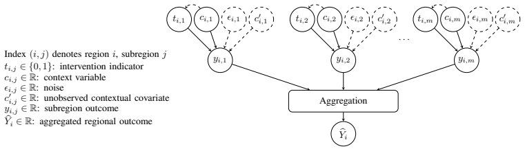
The central object is the shared, invariant structural mechanism $f_\theta(t,c)$—a function that maps a binary treatment indicator and subregional context to a subregional outcome, identical across all regions and subregions—together with the aggregation-consistency training loop. CLAM treats high-resolution context as an auxiliary variable that implicitly defines a prior over high-resolution outcomes, then aggregates the predicted subregional outcomes and enforces agreement with the observed coarse outcome in the loss. The mechanism carries the whole argument: because it is shared, each region's covariate composition provides a different constraint on the same function, and the contrast $f_\theta(1,c)-f_\theta(0,c)$ defines the LOCATE estimand. In restricted variants the aggregation map $g_\phi$ can itself be learned (e.g., a temperature-parameterized softmax interpolating between mean and max aggregation), and latent quantities such as treatment locations or unobserved effect modifiers enter as trainable variables.
What would settle it
Run CLAM on the paper's own non-identifiability example: two regions with subregion contexts (0,1) and (0.5,0.5), both aggregating to the same total, where the constant mechanism and the mechanism $f(c)=c$ are both consistent with the aggregates. If the optimizer reliably selects one mechanism over the other without extra constraints, that selection is inductive bias rather than identification, and a version of the data where the true mechanism is the other one would expose the error.
Extended reading notes
Core claim
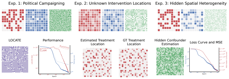
On the paper's own terms, the central discovery is that a high-resolution causal mechanism can be learned from low-resolution supervision when the mechanism is shared across space and the subregional covariates are diverse enough to act as multiple views of the same aggregate outcome. Writing the subregional outcome as $y_{i,j}=f_\theta(t_{i,j},c_{i,j})+\epsilon_{i,j}$ and observing only $\widehat{Y}_i=\sum_j y_{i,j}$ (or another fixed aggregation), CLAM fits $f_\theta$ by minimizing the squared error between the aggregated prediction and the observed regional outcome. The learned mechanism directly yields the local conditional average treatment effect $E_{i,j}=f_\theta(1,c_{i,j})-f_\theta(0,c_{i,j})$, counterfactual outcomes under alternative treatment assignments, and disaggregated outcome maps. The paper demonstrates recovery of heterogeneous effects in a political-campaigning simulation, of latent intervention locations in a school-funding simulation, and of an unobserved spatial effect modifier in a heat-wave experiment; in the real-world heat-and-gun-violence study, CLAM trained on region-level counts produces a temperature–urbanization response surface qualitatively similar to a cell-supervised oracle, though with inflated local magnitudes. The paper does not claim a general identifiability theorem, and states that in a saturated linear view recovery reduces to a rank condition while a prior consistency result for aggregate regression identifies the mechanism only within treatment arms and only where context distributions overlap.
Load-bearing premise
The method requires that a single causal mechanism govern every subregion and that any variation across space be captured by the observed context; if local mechanisms differ in ways that context cannot express, coarse outcomes cannot identify subregional effects.
Editorial extensions
If this is right
- Regional average treatment effects can be computed by aggregating LOCATE over subregions, so coarse-level policy decisions can be informed by predicted local heterogeneity.
- Counterfactual outcomes under alternative intervention placements can be generated by evaluating the learned mechanism on new treatment assignments, enabling subregional 'what if' planning without high-resolution outcome supervision.
- Outcome disaggregation becomes a byproduct: coarse regional outcomes can be mapped to fine-grained predictions whenever the mechanism and the subregional context are available.
- With temporal variation, latent spatial effect modifiers can be recovered from aggregates, as in the heat-wave experiment, provided the functional form is sufficiently constrained.
- An unknown aggregation function can be learned jointly with the local mechanism, as demonstrated when aggregation interpolates between mean and max behavior.
Reading between the lines
- Editorial inference: if CLAM's core claim is right, the ecological fallacy is not only a warning but can be converted into an estimation strategy—compositional variation plus an invariant mechanism is precisely the information that disaggregation needs, suggesting minimal-diversity conditions as a data-design criterion.
- Editorial inference: the overlap limitation implies that LOCATE estimates are only data-supported where treated and untreated subregions share context support; deployments should report overlap diagnostics and restrict causal claims to that support.
- Editorial inference: the inflated local magnitudes seen in the gun-violence case suggest that aggregation-consistency alone is insufficient for calibration, so operational use should combine restart-based diagnostics with external high-resolution validation.
- Editorial inference: the same mechanism principle should transfer to other aggregation domains, such as temporal or administrative-unit aggregation, and to continuous treatments via dose–response curves; a direct test would apply CLAM to time-aggregated outcomes with known fine-scale ground truth.
Editorial analysis
A structured set of objections, weighed in public.
Referee Report
Summary. The paper proposes CLAM, a method for estimating localized causal effects from coarse (region-level) outcomes by combining a shared subregional causal mechanism f_theta(t,c) with high-resolution contextual covariates. Training enforces consistency between the predicted aggregated outcomes and observed low-resolution outcomes, and the learned mechanism is then used to define the local conditional average treatment effect (LOCATE), counterfactual predictions, and outcome disaggregation. The manuscript presents three synthetic experiments (political campaigning, unknown intervention locations, and a spatiotemporal heat-wave study with an unobserved effect modifier), two additional experiments in the appendix (unknown aggregation function and covariate-based confounding), and a semi-synthetic real-world study on temperature and gun violence, where CLAM is trained on aggregated counts and compared against a cell-supervised oracle. The paper also contains an extensive identifiability discussion in Appendix A, explicitly stating that no general identifiability theorem is provided and that LOCATE recovery requires overlap between treated and control context distributions.
Significance. If the central claim is supported, CLAM addresses a practically important problem class: inferring fine-grained causal effects from coarse interventions and outcomes using high-resolution covariates. The paper is commendable for its explicit treatment of assumptions and limitations, for formulating the problem within structural causal models, and for providing reproducible code. The identifiability appendix is unusually honest, distinguishing causal identification, statistical identification from aggregates, and optimizer recovery, and it correctly identifies the overlap condition needed for LOCATE. The synthetic experiments are clean and demonstrate that, under favorable conditions, the aggregate-consistency loss can recover local effects that a uniform disaggregation baseline cannot. However, the significance is tempered by two gaps: no experiment tests the load-bearing overlap/positivity condition, and the experimental evidence for recovering unobserved effect modifiers is limited to a correctly specified linear setting.
major comments (3)
- [§3.3 / Appendix D.3 / Section 7] The stress-test concern about common support lands directly. Appendix A.4 concedes that recovering f0(c) and f1(c) separately identifies LOCATE only where the context distributions of treated and untreated arms overlap, and that outside this overlap a flexible model relies on function-class extrapolation. Yet no experiment tests this condition. In Exp. 1, treatment is assigned randomly and independently of context, so overlap is guaranteed by construction, and the real-world study (Section 6.2, Appendix E) reports no overlap or positivity diagnostics. Because temperature and urbanization are spatially correlated (urban heat islands, seasonality) and no spatial or temporal confounders are modeled, the learned f(temp, urban) may depend on extrapolation. The abstract's claim that CLAM 'reliably captures spatially varying causal effects across diverse settings' is therefore unsupported. Please add a synthetic experiment with deliberately limited or absent overlap between treatment arms, report support diagnostics (e.g., estimated densities of context under each arm) in the real-world study, and qualify the abstract and conclusions accordingly.
- [Section 6.2 / Appendix E / Section 8] The claim that CLAM can reconstruct unobserved spatial effect modifiers is not established at the level asserted in Section 3.3. In Exp. 3, the latent vegetation matrix U is fitted using the same aggregate outcomes that supervise the mechanism f_theta, and the MLP variant yields substantially higher vegetation MSE than the linear variant. The paper itself notes that the MLP can absorb transformations of U while preserving aggregated predictions, which is an identifiability trade-off rather than evidence of a general capability. The linear variant succeeds only because it matches the true mechanism. Please either provide an identifiability condition under which temporal variation constrains the latent variable (as hinted in Appendix A.5), or present Exp. 3 as a proof-of-concept under correct specification and remove or qualify the broader claim in Section 3.3 that temporal variation 'supplies enough constraints'.
- [Abstract / Section 8] The real-world study's systematic overestimation of local magnitudes is acknowledged as an aggregation-induced identifiability gap, but the paper's framing does not match this evidence. Section 6.2 and Appendix E report inflated peak intensities and broader spatial support relative to the cell-supervised oracle, and Section 8 concludes that 'absolute local magnitudes may be systematically overestimated.' Yet the abstract states that CLAM 'reliably captures spatially varying causal effects' and 'principled outcome disaggregation' across diverse settings, which is too strong given the reported behavior. Please revise the abstract and introduction to state that relative structure and causal dependencies can be recovered, while absolute local magnitudes may be biased without fine-grained outcome supervision.
minor comments (6)
- [Figure 5] The phrase 'without loss of generality' for assuming identical subregion structure, binary treatments, and scalar variables is a modeling simplification, not a genuine WLOG reduction; please rephrase to 'for simplicity' or 'for clarity of exposition.'
- [Appendix D.3] The heading 'LOACATE MAE' contains a typo and should read 'LOCATE MAE.'
- [Appendix E] The results for Exp. 3 refer to a 'linear scaling parameterization' and an MLP, but the training subsection only specifies the MLP architecture; please explicitly define the linear variant, including its parameters and how it is optimized.
- [Appendix D.1] Equation (10) uses epsilon both in the denominator (to avoid division by zero) and as a stabilization constant in the loss in Equation (14); please define distinct symbols or clarify the roles of these constants.
- [Section 3.4] The piecewise linear function interp(c) is defined only on the interval [-2,1], but contexts are sampled from a standard Gaussian and can fall outside this range; please state whether extrapolation is intended and how it is performed.
- [Section 8] The reference to 'consistency analysis of Zhang et al. [12]' would benefit from a brief statement of what that consistency result guarantees, since the main text currently defers all details to Appendix A.
Circularity Check
No significant circularity: LOCATE is a post-training contrast of the learned mechanism, not a term in the aggregate loss, and the paper's supporting identification argument relies on an external result rather than on self-citation.
full rationale
The central estimand LOCATE is defined in Eq. (4) as E_{i,j}=f_theta(1,c_{i,j})-f_theta(0,c_{i,j}) after training, while the training objective in Section 3.2 is only the MSE between observed and predicted regional aggregates; LOCATE never appears in the loss, so it is not baked into the fit by construction. The mechanism f_theta is shared across subregions and its identification from aggregates is supported by the external consistency result of Zhang et al. [12] (Appendix A.4), not by a self-citation. The paper explicitly disclaims a general identifiability theorem (Section 3.4) and concedes that LOCATE is identified only where treated and control context distributions overlap, and that outside this overlap a flexible model relies on function-class extrapolation (Appendix A.4); this is an honest limitation rather than a circular reduction. Experiment 3's latent vegetation field is fitted on the same aggregate outcomes used to fit the mechanism, but the paper itself reports that MLP recovery is fragile and attributes this to an identifiability gap, so it is not presenting a fitted parameter as an independent prediction. The real-world study uses an oracle trained on high-resolution counts only as an evaluation reference, not as a CLAM output. The only author-overlapping citation is [16] (Vollmer as co-author), used to motivate a time-varying-confounding extension; it is not load-bearing. No equation reduces to its own input, and no load-bearing claim is justified solely by a self-citation chain.
Assumptions & free parameters
free parameters (5)
- Neural network weights theta of f_theta (Exp. 1, 3, real-world study) =
learned from aggregate loss
- Latent treatment logits (Exp. 2) =
N x M trainable logits, Gumbel-Softmax annealed from 2.0 to 0.1
- Latent vegetation matrix U (Exp. 3) =
N x M values in [0,1], learned
- Aggregation temperature tau (Exp. 4) =
approximately 6 for mean case, approximately 5.6 for max case
- Confounding allocation parameters beta_0, beta_1, tau_conf (Exp. 5) =
learned
assumptions (8)
- domain assumption Single invariant causal mechanism f_theta(t,c) shared across subregions and regions
- domain assumption No hidden confounding, and treatment assignment independent of context in the baseline setting
- domain assumption Known aggregation function in the main setting (sum/mean), with unknown aggregation restricted to a one-parameter softmax in Exp. 4
- domain assumption Treatment is assigned at region level and inherited by all subregions
- domain assumption Context covariates are exogenous, not caused by treatment or outcome, in the baseline motif
- domain assumption Sufficient diversity in subregional covariate compositions across regions
- standard math Backdoor criterion is valid for LOCATE under the assumed graph
- standard math Zhang et al. [12] consistency result for learning from aggregate observations
Cite this review
Pith. "Pith review of CLAM: Causal Spatial Disaggregation to Infer Local Effects From Coarse Data." pith.science (2026). https://pith.science/paper/UPNLCRIP
@misc{pith2026260808064,
  author       = {Pith},
  title        = {Pith review of: CLAM: Causal Spatial Disaggregation to Infer Local Effects From Coarse Data},
  year         = {2026},
  howpublished = {\url{https://pith.science/paper/UPNLCRIP}},
  note         = {Machine review of arXiv:2608.08064}
}
read the original abstract
Learning fine-grained spatial patterns from coarse-resolution data is challenging, especially in causal settings where high-resolution effects must be inferred from aggregated interventions and outcomes. We introduce CLAM, a method for estimating localized causal effects from coarse observations by exploiting high-resolution contextual covariates that modulate these effects. By jointly learning the causal mechanism and a disaggregation mapping, CLAM captures interactions that are missed when addressing these problems independently. The method supports localized effect estimation, counterfactual reasoning, and principled outcome disaggregation, and reliably captures spatially varying causal effects across diverse settings. This is particularly relevant for applications such as public health and environmental policy, where decisions are made at broad scales despite substantial local heterogeneity. Code is available at https://github.com/gerritgr/clam
Figures

Figures from the paper (9 more)


Reference graph
Works this paper leans on
-
[1]
A systematic review of spatial disaggregation methods for climate action planning.Energy and AI, 17:100386, 2024
Shruthi Patil, Noah Pflugradt, Jann M Weinand, Detlef Stolten, and Jürgen Kropp. A systematic review of spatial disaggregation methods for climate action planning.Energy and AI, 17:100386, 2024
2024
-
[2]
Yongjian Sun, Kefeng Deng, Kaijun Ren, Jia Liu, Chongjiu Deng, and Yongjun Jin. Deep learning in statistical downscaling for deriving high spatial resolution gridded meteorological data: A systematic review.ISPRS Journal of Photogrammetry and Remote Sensing, 208:14–38, 2024
2024
-
[3]
Ecological inference.Proceedings of the National Academy of Sciences, 96(19): 10578–10581, 1999
Alexander A Schuessler. Ecological inference.Proceedings of the National Academy of Sciences, 96(19): 10578–10581, 1999
1999
-
[4]
A deep journey into super-resolution: A survey.ACM computing surveys (CSUR), 53(3):1–34, 2020
Saeed Anwar, Salman Khan, and Nick Barnes. A deep journey into super-resolution: A survey.ACM computing surveys (CSUR), 53(3):1–34, 2020
2020
-
[5]
On the modern deep learning approaches for precipitation downscaling.Earth Science Informatics, 16(2):1459–1472, 2023
Bipin Kumar, Kaustubh Atey, Bhupendra Bahadur Singh, Rajib Chattopadhyay, Nachiketa Acharya, Manmeet Singh, Ravi S Nanjundiah, and Suryachandra A Rao. On the modern deep learning approaches for precipitation downscaling.Earth Science Informatics, 16(2):1459–1472, 2023
2023
-
[6]
Downscaling spatial structure for the analysis of epidemiological data.Computers, Environment and Urban Systems, 32(1):81–93, 2008
Timothy C Matisziw, Tony H Grubesic, and Hu Wei. Downscaling spatial structure for the analysis of epidemiological data.Computers, Environment and Urban Systems, 32(1):81–93, 2008
2008
-
[7]
Integrating big social data, computing and modeling for spatial social science, 2016
Xinyue Ye, Qunying Huang, and Wenwen Li. Integrating big social data, computing and modeling for spatial social science, 2016
2016
-
[8]
Cambridge university press, 2009
Judea Pearl.Causality. Cambridge university press, 2009
2009
Show all 87 references
-
[9]
Abstracting causal models
Sander Beckers and Joseph Y Halpern. Abstracting causal models. InProceedings of the aaai conference on artificial intelligence, volume 33, pages 2678–2685, 2019
2019
-
[10]
Deep sets.Advances in neural information processing systems, 30, 2017
Manzil Zaheer, Satwik Kottur, Siamak Ravanbakhsh, Barnabas Poczos, Russ R Salakhutdinov, and Alexander J Smola. Deep sets.Advances in neural information processing systems, 30, 2017
2017
-
[11]
Neural message passing for quantum chemistry
Justin Gilmer, Samuel S Schoenholz, Patrick F Riley, Oriol Vinyals, and George E Dahl. Neural message passing for quantum chemistry. InInternational conference on machine learning, pages 1263–1272. Pmlr, 2017
2017
-
[12]
Learning from aggregate observations.Advances in Neural Information Processing Systems, 33:7993–8005, 2020
Yivan Zhang, Nontawat Charoenphakdee, Zhenguo Wu, and Masashi Sugiyama. Learning from aggregate observations.Advances in Neural Information Processing Systems, 33:7993–8005, 2020
2020
-
[13]
Abstraction between structural causal models: A review of definitions and properties.arXiv preprint arXiv:2207.08603, 2022
Fabio Massimo Zennaro. Abstraction between structural causal models: A review of definitions and properties.arXiv preprint arXiv:2207.08603, 2022
2022 arXiv
-
[14]
Jonas Peters, Peter Bühlmann, and Nicolai Meinshausen. Causal inference by using invariant prediction: identification and confidence intervals.Journal of the Royal Statistical Society Series B: Statistical Methodology, 78(5):947–1012, 2016
2016
-
[15]
Toward causal representation learning.Proceedings of the IEEE, 109(5): 612–634, 2021
Bernhard Schölkopf, Francesco Locatello, Stefan Bauer, Nan Rosemary Ke, Nal Kalchbrenner, Anirudh Goyal, and Yoshua Bengio. Toward causal representation learning.Proceedings of the IEEE, 109(5): 612–634, 2021
2021
-
[16]
Model updating after interventions paradoxically introduces bias
James Liley, Samuel Emerson, Bilal Mateen, Catalina Vallejos, Louis Aslett, and Sebastian V ollmer. Model updating after interventions paradoxically introduces bias. InInternational Conference on Artificial Intelligence and Statistics, pages 3916–3924. PMLR, 2021
2021
-
[17]
Statistical downscaling for climate science
Douglas Maraun. Statistical downscaling for climate science. InOxford Research Encyclopedia of Climate Science. 2019
2019
-
[18]
Deconditional downscaling with gaussian processes
Siu Lun Chau, Shahine Bouabid, and Dino Sejdinovic. Deconditional downscaling with gaussian processes. Advances in Neural Information Processing Systems, 34:17813–17825, 2021
2021
-
[19]
Effectiveness of causality- based predictor selection for statistical downscaling: a case study of rainfall in an ecuadorian andes basin
Angel Vázquez-Patiño, Esteban Samaniego, Lenin Campozano, and Alex Avilés. Effectiveness of causality- based predictor selection for statistical downscaling: a case study of rainfall in an ecuadorian andes basin. Theoretical and Applied Climatology, 150(3):987–1013, 2022
2022
-
[20]
Riya Dutta and Rajib Maity. Identification of potential causal variables for statistical downscaling models: effectiveness of graphical modeling approach.Theoretical and Applied Climatology, 142(3):1255–1269, 2020. 11
2020
-
[21]
Ecological inference and the ecological fallacy.International Encyclopedia of the social & Behavioral sciences, 6(4027-4030):1–7, 1999
David A Freedman. Ecological inference and the ecological fallacy.International Encyclopedia of the social & Behavioral sciences, 6(4027-4030):1–7, 1999
1999
-
[22]
Aggregation and disaggregation techniques and methodology in optimization.Operations research, 39(4):553–582, 1991
David F Rogers, Robert D Plante, Richard T Wong, and James R Evans. Aggregation and disaggregation techniques and methodology in optimization.Operations research, 39(4):553–582, 1991
1991
-
[23]
Hierarchical causal models.Journal of Machine Learning Research, 27(37):1–73, 2026
Eli N Weinstein and David M Blei. Hierarchical causal models.Journal of Machine Learning Research, 27(37):1–73, 2026
2026
-
[24]
Spatio-temporal hierarchical causal models
Xintong Li, Haoran Zhang, and Xiao Zhou. Spatio-temporal hierarchical causal models. InProceedings of the AAAI Conference on Artificial Intelligence, volume 40, pages 23230–23238, 2026
2026
-
[25]
Approximate causal abstractions
Sander Beckers, Frederick Eberhardt, and Joseph Y Halpern. Approximate causal abstractions. In Uncertainty in artificial intelligence, pages 606–615. PMLR, 2020
2020
-
[26]
Toward causal inference for spatio-temporal data: Conflict and forest loss in colombia.Journal of the American Statistical Association, 117(538):591–601, 2022
Rune Christiansen, Matthias Baumann, Tobias Kuemmerle, Miguel D Mahecha, and Jonas Peters. Toward causal inference for spatio-temporal data: Conflict and forest loss in colombia.Journal of the American Statistical Association, 117(538):591–601, 2022
2022
-
[27]
Lingxiao Zhou, Kosuke Imai, Jason Lyall, and Georgia Papadogeorgou. Estimating heterogeneous treatment effects for spatio-temporal causal inference: How economic assistance moderates the effects of airstrikes on insurgent violence.arXiv preprint arXiv:2412.15128, 2024
2024 arXiv
-
[28]
Spatiotemporal causal inference with arbitrary spillover and carryover effects.arXiv preprint arXiv:2504.03464, 2025
Mitsuru Mukaigawara, Kosuke Imai, Jason Lyall, and Georgia Papadogeorgou. Spatiotemporal causal inference with arbitrary spillover and carryover effects.arXiv preprint arXiv:2504.03464, 2025
2025
-
[29]
Bipartite causal inference with interference, time series data, and a random network.arXiv preprint arXiv:2404.04775, 2024
Zhaoyan Song and Georgia Papadogeorgou. Bipartite causal inference with interference, time series data, and a random network.arXiv preprint arXiv:2404.04775, 2024
2024 arXiv
-
[30]
Gst-unet: A neural framework for spatiotemporal causal inference with time-varying confounding.Advances in Neural Information Processing Systems, 38:17295–17322, 2026
Miruna Oprescu, David Park, Xihaier Luo, Shinjae Yoo, and Nathan Kallus. Gst-unet: A neural framework for spatiotemporal causal inference with time-varying confounding.Advances in Neural Information Processing Systems, 38:17295–17322, 2026
2026
-
[31]
Causal discovery on vector-valued variables and consistency-guided aggregation.arXiv preprint arXiv:2505.10476, 2025
Urmi Ninad, Jonas Wahl, Andreas Gerhardus, and Jakob Runge. Causal discovery on vector-valued variables and consistency-guided aggregation.arXiv preprint arXiv:2505.10476, 2025
2025 arXiv
-
[32]
The causal effects of modified treatment policies under network interference.arXiv preprint arXiv:2412.02105, 2024
Salvador V Balkus, Scott W Delaney, and Nima S Hejazi. The causal effects of modified treatment policies under network interference.arXiv preprint arXiv:2412.02105, 2024
2024 arXiv
-
[33]
Invariant causal prediction for nonlinear models.Journal of Causal Inference, 6(2):20170016, 2018
Christina Heinze-Deml, Jonas Peters, and Nicolai Meinshausen. Invariant causal prediction for nonlinear models.Journal of Causal Inference, 6(2):20170016, 2018
2018
-
[34]
Invariant models for causal transfer learning.Journal of Machine Learning Research, 19(36):1–34, 2018
Mateo Rojas-Carulla, Bernhard Schölkopf, Richard Turner, and Jonas Peters. Invariant models for causal transfer learning.Journal of Machine Learning Research, 19(36):1–34, 2018
2018
-
[35]
Hierarchical models for causal effects.Emerging trends in the social and behavioral sciences, 1:16, 2015
Avi Feller and Andrew Gelman. Hierarchical models for causal effects.Emerging trends in the social and behavioral sciences, 1:16, 2015
2015
-
[36]
A hierarchical model for aggregated functional data.Technometrics, 55(3):321–334, 2013
Ronaldo Dias, Nancy L Garcia, and Alexandra M Schmidt. A hierarchical model for aggregated functional data.Technometrics, 55(3):321–334, 2013
2013
-
[37]
Ecological regressions and behavior of individuals.American sociological review, 18(6): 663, 1953
Leo A Goodman. Ecological regressions and behavior of individuals.American sociological review, 18(6): 663, 1953
1953
-
[38]
Gun violence archive gva
Gun Violence Archive. Gun violence archive gva. Web Archive, 2015. URL https: //www.loc.gov/item/lcwaN0016293/. United States. Retrieved from Library of Congress: https://www.loc.gov/item/lcwaN0016293/
2015
-
[39]
Analysis of daily ambient temperature and firearm violence in 100 us cities.JAMA network open, 5(12):e2247207– e2247207, 2022
Vivian H Lyons, Emma L Gause, Keith R Spangler, Gregory A Wellenius, and Jonathan Jay. Analysis of daily ambient temperature and firearm violence in 100 us cities.JAMA network open, 5(12):e2247207– e2247207, 2022
2022
-
[40]
Fay and Roger A
Robert E. Fay and Roger A. Herriot. Estimates of income for small places: an application of James-Stein procedures to census data.Journal of the American Statistical Association, 74(366):269–277, 1979
1979
-
[41]
A review of spatial downscaling of satellite remotely sensed soil moisture.Reviews of Geophysics, 55(2):341–366, 2017
Jian Peng, Alexander Loew, Olivier Merlin, and Niko EC Verhoest. A review of spatial downscaling of satellite remotely sensed soil moisture.Reviews of Geophysics, 55(2):341–366, 2017
2017
-
[42]
Gotway and Linda J
Carol A. Gotway and Linda J. Young. Combining incompatible spatial data.Journal of the American Statistical Association, 97(458):632–648, 2002. 12
2002
-
[43]
Lucas, Seth Flaxman, Katherine Battle, and Kenji Fukumizu
Ho Chung Leon Law, Dino Sejdinovic, Ewan Cameron, Tim C.D. Lucas, Seth Flaxman, Katherine Battle, and Kenji Fukumizu. Variational learning on aggregate outputs with Gaussian processes. InAdvances in Neural Information Processing Systems, 2018
2018
-
[44]
Robinson
William S. Robinson. Ecological correlations and the behavior of individuals.American Sociological Review, 15(3):351–357, 1950
1950
-
[45]
Princeton University Press, 1997
Gary King.A Solution to the Ecological Inference Problem: Reconstructing Individual Behavior from Aggregate Data. Princeton University Press, 1997
1997
-
[46]
Inferring causation from time series in earth system sciences.Nature communications, 10(1):2553, 2019
Jakob Runge, Sebastian Bathiany, Erik Bollt, Gustau Camps-Valls, Dim Coumou, Ethan Deyle, Clark Glymour, Marlene Kretschmer, Miguel D Mahecha, Jordi Muñoz-Marí, et al. Inferring causation from time series in earth system sciences.Nature communications, 10(1):2553, 2019. A Iden...
2019
-
[47]
For the linear model in Equation (3), identification reduces to a rank condition on the aggregate design matrix
-
[48]
mean-aggregation special case connects directly to the functional consistency result of Zhang et al
For the additive model in Equation (2), the i.i.d. mean-aggregation special case connects directly to the functional consistency result of Zhang et al. [12]. Within each treatment arm, their result identifies the conditional-mean function almost everywhere under the correspond...
-
[49]
Recovery in these regimes is studied empirically and remains an important theoretical problem
For the general model in Equation (1), including dependent spatial designs, structured latent variables, unknown or nonlinear aggregation, and extrapolation outside the observed treatment–context support, we do not claim a general identification theorem. Recovery in these regi...
-
[50]
The aggregation functiong ϕ(·)is consistent and applied uniformly across regions
-
[51]
The observed covariate compositions {ci,j}M j=1 differ across regions, which induces identifi- able variation in the aggregates bYi under the shared mechanismf θ(·). Given sufficient diversity and the assumption of causal invariance, the aggregated outputs provide a supervisor...
-
[52]
Initializing all entries to zero
-
[53]
Randomly selecting50%of the regions for treatment
-
[54]
, M}uniformly at random and assigningt i,j = 1
For each treated region i, choosing exactly one subregion j∈ {1, . . . , M}uniformly at random and assigningt i,j = 1. The context matrixCis sampled i.i.d. from a standard normal distribution: ci,j ∼ N(0,1). The outcome variable is given by the ground-truth functional relation...
-
[55]
Sample a mini-batch of region indices
-
[56]
Process the latent treatment logits using the Gumbel-Softmax relaxation to obtain an estimate of the high-resolution treatment matrixTfor the mini-batch
-
[57]
Compute predicted subregional outcomes: µi,j =f θ bti,j, ci,j
-
[58]
Aggregate to regional predictions by summation: µi = MX j=1 µi,j
-
[59]
heat waves
Compare the regional prediction with the observed regional outcome bYi using the MSE loss. We optimize all parameters jointly using AdamW with learning rate 10−4. Training is performed for 200,000epochs with a fixed random seed. 23 Details of Exp. 3: Spatiotemporal Effects of ...
-
[60]
The mapping fθ(·) from observed context, intervention, and vegetation index to subregional outcomes,
-
[61]
The function fθ(·) is implemented as a 4 layer multilayer perceptron (MLP) with hidden dimension 16and a dropout rate of0.1after the second hidden layer
The static vegetation index valuesU∈[0,1] N×M for all subregions. The function fθ(·) is implemented as a 4 layer multilayer perceptron (MLP) with hidden dimension 16and a dropout rate of0.1after the second hidden layer. Its inputs for each subregion are: z(w) i,j = 1[c(w) i,j ...
-
[62]
The model takes as inputT (w),C (w), andU,
-
[63]
The MLP evaluatesf θ(·)at each(i, j)to produce predicted subregional outcomesy (w) i,j , 25
-
[64]
These are aggregated to the regional level via mean aggregation
-
[65]
Training proceeds over all months in random order at each epoch
The primary loss is the MSE between predicted and observed regional outcomes. Training proceeds over all months in random order at each epoch. The total parameter set consists of the MLP weights θ and the vegetation matrix U. We optimize using Adam with a learning rate of 0.00...
-
[66]
Both training loss and MSE decrease rapidly, and the final error is very small, indicating near-perfect recovery of the unobserved covariate
Figure 8a shows the loss curves and vegetation MSE under the linear scaling parameter- ization. Both training loss and MSE decrease rapidly, and the final error is very small, indicating near-perfect recovery of the unobserved covariate
-
[67]
The two maps are almost indistinguishable, confirming that the restricted functional form matches the data-generating process and allows highly accurate recovery
Figure 8b compares the ground-truth vegetation field to the estimated vegetation under linear scaling. The two maps are almost indistinguishable, confirming that the restricted functional form matches the data-generating process and allows highly accurate recovery
-
[68]
Figures 8c and d present the same results for the non-linear MLP parameterization. While the model still recovers meaningful structure in the vegetation, the MSE remains orders of magnitude higher than in the linear case, and deviations from the ground truth are clearly visibl...
-
[69]
Overall, these results demonstrate that the model can reconstruct regional outcomes while also uncovering hidden drivers of heterogeneity. The comparison between linear and non- linear parameterizations highlights the trade-off: structural restrictions yield more accurate reco...
-
[70]
The parametersθ={θ base, θveg}of the causal effect functionf θ(·),
-
[71]
The learned function takes the form: fθ(ti,j, ci,j) = 0.0ift i,j = 0, θbase +θ veg ·c i,j ift i,j = 1
The aggregation temperature parameter τ >0 governing the softmax-based aggregation from subregional to regional outcomes. The learned function takes the form: fθ(ti,j, ci,j) = 0.0ift i,j = 0, θbase +θ veg ·c i,j ift i,j = 1. In the forward pass:
-
[72]
Compute predicted subregional outcomes:y i,j =f θ(ti,j, ci,j),
-
[73]
Compute subregion-level aggregation weights via the softmax: pi,j(τ) = exp (yi,j /τ)PM k=1 exp (yi,k/τ) ,
-
[74]
Compute predicted regional outcomes as the expectation under pi,j(τ): yi = PM j=1 pi,j(τ)· yi,j,
-
[75]
All parameters {θbase, θveg, τ}are optimized jointly using Adam with a learning rate of 0.001 for 1000 epochs
Compute the loss as the mean squared error with the observedY i. All parameters {θbase, θveg, τ}are optimized jointly using Adam with a learning rate of 0.001 for 1000 epochs. We initialize τ to a moderate value (e.g., τ= 1.0) and enforce τ >0 during training by optimizing its...
-
[76]
Visualizations of the aggregated causal effects show that mean aggregation preserves more variation across regions, whereas max aggregation suppresses smaller effects and produces sharper contrasts
-
[77]
Training loss is substantially higher under max aggregation, as weaker subregional signals are obscured
Although the subregional causal effect loss is never used directly for training, it decreases steadily over epochs, indicating that the model recovers fine scale effects from only re- gional supervision. Training loss is substantially higher under max aggregation, as weaker su...
-
[78]
Comparing estimated and ground truth local effects confirms this bias: areas with small true effects tend to be overestimated when max aggregation dominates
-
[79]
The aggregation function, parameterized by the temperature τ, is recovered with high accuracy. In the mean aggregation case, τ is estimated within 0.01 of the ground truth, while in the max aggregation case, the estimate is slightly underestimated (5.6), consistent with the pl...
-
[80]
Overall, the experiment demonstrates that our approach can successfully recover both the aggregation mechanism (within its parametric form) and the underlying causal effects, despite only observing region-level outcomes. F.2 Exp. 5: Covariate-Based Confounding of Treatment Sub...
-
[81]
Treats the treatment allocation as if independent of the context,
-
[82]
Learns T as free parameters, constrained to be one hot per row via a differentiable argmax with temperature,
-
[83]
This ignores the fact that the treatment assignment mechanism is context dependent
Learnsθby minimizing the MSE between observed and predicted regional outcomes. This ignores the fact that the treatment assignment mechanism is context dependent. Regime 2: Confounding Aware Training.Here, we explicitly model the context-dependent treatment allocation mechanis...
-
[84]
The aggregated causal effects differ markedly depending on the level of confounding, showing that the treatment context dependency directly shapes the observed regional outcomes
We compare two cases of confounding in subregional treatment allocation, holding region- level treatments and contextual factors fixed. The aggregated causal effects differ markedly depending on the level of confounding, showing that the treatment context dependency directly s...
-
[85]
Under strong confounding, the confounding- aware approach recovers the true intervention locations with high fidelity, while the naïve method from Exp
We visualize the ground truth intervention locations alongside the estimates obtained with and without explicitly modeling confounding. Under strong confounding, the confounding- aware approach recovers the true intervention locations with high fidelity, while the naïve method...
-
[86]
This confirms that adjusting for confounding does not reduce performance when confounding is weak
In the low confounding setting, both methods perform similarly, and location probabilities are estimated with comparable accuracy. This confirms that adjusting for confounding does not reduce performance when confounding is weak
-
[87]
Under high confounding, the respective errors were 0.74 versus 0.32
For causal effect estimation, the final MSE of subregional effects under low confounding was 2.04 (naïve) versus 1.60 (confounding aware). Under high confounding, the respective errors were 0.74 versus 0.32. These results show that accounting for confounding improves both inte...
Reviewed August 12, 2026 · model on record in the stance chip above.
Discussion (0). Continue with ORCID to comment.