REVIEW 5 major objections 4 minor 39 references
Generative Models: Principles, Architectures, and Applications
T0 review · 5 major / 4 minor · reviewed 2026-08-12 · deepseek-v4-flash
Pith's one-line read This book claims all of generative AI—VAEs, GANs, diffusion, flow matching, and sampling—can be taught as one coherent distribution-transformation subject, from ELBO math to Stable Diffusion 3.
desk verdict A useful, comprehensive textbook-style review of generative modeling whose organizational framing is genuinely helpful, but internal math errors in the foundations need fixing before it can be trusted as a self-contained resource. read the letter →
The pith
A machine-rendered reading of the paper's core claim, the machinery that carries it, and where it could break.
The reading
What carries the argument
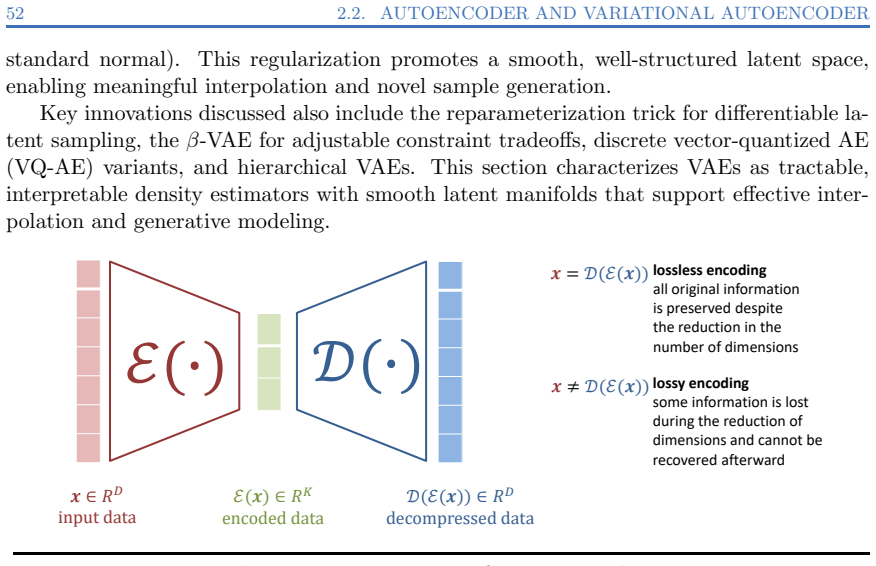
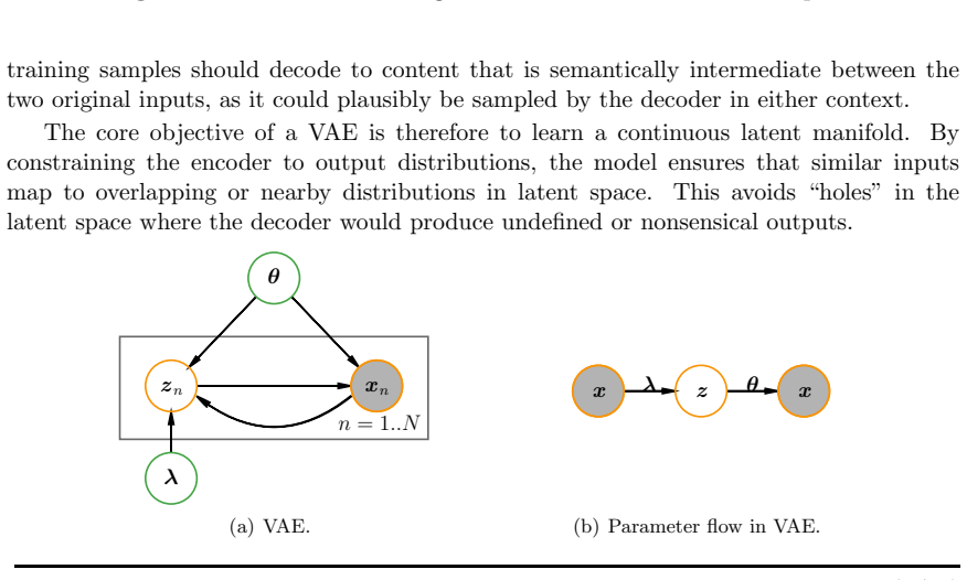
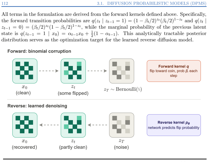
The load-bearing objects are the evidence lower-bound and the distribution-transformation framing. The book develops $\mathrm{ELBO} = \ln p_\theta(\mathbf{x}) - D_{\mathrm{KL}}[q \| p_\theta(\cdot|\mathbf{x})]$ as the shared objective for VAEs, EM, and diffusion models; forward and reverse noising processes $q(\mathbf{x}_t|\mathbf{x}_0)$ for diffusion and score-based models; conditional and marginal probability paths with vector fields for flow matching; and exponential-integrator solvers for accelerated sampling. The ELBO decomposition $\ln p_\theta(\mathbf{X}) = \mathrm{ELBO} + D_{\mathrm{KL}}[q \| p_\theta(\mathbf{z}|\mathbf{x})]$ is the recurring identity that connects variational inference, EM's E-step, and diffusion training objectives throughout the book.
What would settle it
Verify that Theorem 1.5's proof of spectral decomposition can be reconstructed using only the material printed in this book's Chapter 1; if the proof is not recoverable without consulting Lu (2021a), the self-contained mathematical promise is falsified. As a second concrete test, implement the GMM EM derivation of Example 2.2 on a two-component toy dataset: if the described Q-function maximization does not converge to the known maximum-likelihood solution, the derivation chain is broken.
Extended reading notes
Core claim
On the author's terms, the central claim is pedagogical and conceptual: generative modeling is not a zoo of unrelated tricks but a small set of connected ideas organized under the distribution-transformation framing. Concretely, the book asserts that GANs, VAEs, normalizing flows, diffusion models, score-based models, and flow matching all learn a deterministic or stochastic map from a simple tractable prior (typically the standard Gaussian) to the target data distribution, and that their training objectives are unified through the ELBO, KL divergence, and conditional/marginal probability paths. It further claims that this organization is accurate and complete enough to guide a reader from foundational probability and linear algebra to state-of-the-art systems, including Stable Diffusion 3, and to advanced sampling algorithms such as DEIS, DPM-Solver, and DPM-Solver++.
Load-bearing premise
The book's promise of self-contained mathematical underpinnings rests on the correctness and availability of the author's earlier texts, since foundational proofs (spectral decomposition, SVD existence, Woodbury identity) are deferred to those references rather than proved in this book.
Editorial extensions
If this is right
- A reader who follows the ELBO derivations through Chapters 2 and 3 can derive the VAE loss, the EM Q-function, and the DDPM noise-prediction objective as special cases of the same lower-bound argument.
- Diffusion models are presented as three equivalent views—denoising prediction, score matching, and SDE/ODE solving—so tools developed for one view transfer to the others.
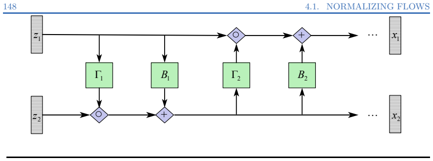
- Flow matching and normalizing flows are shown as complementary frameworks that offer exact likelihoods and stable training, unified with diffusion under the same transport picture.
- Modern architectures (U-Net, ControlNet, DiT, multimodal DiT) and guidance mechanisms (classifier and classifier-free) are presented as modular components of the distribution-transformation framework, not as isolated innovations.
- Advanced samplers such as DPM-Solver and DPM-Solver++ drastically reduce the number of function evaluations while preserving fidelity, addressing the main computational bottleneck of iterative diffusion sampling.
Reading between the lines
- The book leaves implicit that its distribution-transformation view is model-family-agnostic, so a sampler derived for diffusion (e.g., DPM-Solver) should in principle apply to any learned velocity field, including flow-matching models; the derivations give the reader the tools to test that claim directly.
- The book's ELBO-first progression suggests a testable pedagogical hypothesis: teaching diffusion models after ELBO-based VAEs makes them easier to learn than an adversarial-first curriculum. This could be evaluated through a learning-outcome study comparing the two orderings.
- The book's promise of self-contained mathematics is contingent on the availability and correctness of the author's earlier texts, since foundational proofs—spectral decomposition, SVD existence, and Woodbury's identity—are deferred to those references rather than proved here.
- A practical reading strategy implied by the book is to verify Exercise 1.7 (SVD existence) independently before relying on later chapters, since the SVD theorem underlies the PCA/linear-autoencoder equivalence developed in Chapter 2.
Signed reviews
Editorial analysis
A structured set of objections, weighed in public.
Referee Report
Summary. This manuscript is a textbook-length exposition of generative modeling, spanning mathematical preliminaries, latent-variable models (VAEs and GANs), diffusion models, flow matching, score-based methods, advanced samplers, and modern generative architectures. Its stated aim, in the preface, is to guide readers through the foundational principles, mathematical underpinnings, and practical architectures of generative AI. The book is organized as a sequence of chapters with embedded definitions, theorems, examples, and problem sets. The core derivations for the ELBO, EM, VAE losses, and diffusion objectives follow the standard literature, but the manuscript also contains several incorrect mathematical statements in its foundational chapters and exercises.
Significance. The book has genuine pedagogical value if corrected: the topic selection is comprehensive, the progression from ELBO/EM to VAEs and diffusion models is sensible, and many of the derivations are standard and clearly motivated. I credit the manuscript for attempting to connect classical variational inference to modern deep generative models and for including exercise problems that ask readers to prove key results. However, the book's central claim of providing the mathematical underpinnings of generative models is directly undermined by internal errors in Chapter 1 and Section 2.1.4, which are prerequisites for the rest of the text. Since these are errors in the manuscript itself rather than merely deferred citations, they are load-bearing for the pedagogical promise. The manuscript does not include machine-checked proofs or reproducible code, so its value rests on the correctness of its mathematical exposition.
major comments (5)
- [§2.1.4, Eq. (2.18)] The mean-field ELBO expansion is incorrect as written. The displayed formula writes the integrand as ∏_q q_{znq}(z_{nq}) ln pθ(zn,xn) − Σ_q q_{znq}(z_{nq}) ln q_{znq}(z_{nq}), integrated over dzn. Because dzn is the full latent vector, the entropy term must involve the full product ∏_q q_{znq}(z_{nq}) multiplying each ln q_{znq}(z_{nq}); equivalently the correct integrand is (∏_q q_{znq}) [ln pθ(zn,xn) − Σ_q ln q_{znq}(z_{nq})]. The printed sum without the product cannot arise from the preceding line and would mislead any reader trying to derive the mean-field coordinate ascent updates.
- [§1.2.5, Figure 1.6] The example G(x,y)=√(x²+y²) claims that directional derivatives exist at the origin for directions d=[a,b]^T with a,b≠0, but the defining limit from Definition 1.16 is lim_{μ→0} (|μ|√(a²+b²))/μ, whose one-sided limits are +√(a²+b²) and −√(a²+b²). The two-sided limit therefore does not exist for any nonzero direction d. This example does not illustrate the intended phenomenon; it actually contradicts Definition 1.16 and needs to be corrected.
- [Chapter 1 Problem 1.4, Eq. (1.36)] The univariate joint Gaussian likelihood contains N·Sx in the exponent, where Sx = Σ_{n=1}^N (x_n − ar x)². The correct decomposition is exp(−(1/(2σ²))[N(ar x−μ)² + Sx]); the second term should be Sx, not N·Sx. This is inconsistent with the multivariate formula displayed immediately below, which correctly uses tr(Σ^{−1}Sx) without an extra factor of N in the second exponential term.
- [Chapter 1 Problem 1.8] Parts (a) and (b) state E[x|y] = x when x is independent of y, and E[c|x] = x for a constant c. Both statements are wrong: the first should be E[x|y] = E[x] (a constant random variable), and the second should be E[c|x] = c. As printed, the exercise contradicts the unbiasedness property E[E[x|y]] = E[x] derived in Eq. (1.25) and teaches the opposite of the defining property of conditional expectation.
- [§1.2.5, Theorem 1.21] The quadratic approximation theorem is stated under the hypothesis that f is twice continuously differentiable, but the claim includes an O(∥y−x∥³) remainder term. Under only C² regularity, the sharp Taylor remainder is o(∥y−x∥²); the O(∥d∥³) bound requires third-order differentiability and is not a consequence of the stated hypothesis. The statement either needs a stronger hypothesis or a corrected remainder order.
minor comments (4)
- [Notation, Functions table] The notation table lists both ∥x∥=∥x∥1 and ∥x∥=∥x∥∞ for the same symbol ∥x∥, while Section 1.2.1 explicitly sets the convention ∥x∥=∥x∥₂. This shorthand should be made consistent or the table entries should be corrected.
- [§1.2.5, Theorem 1.20] The result labeled 'Linear approximation theorem' is actually a second-order Taylor expansion with Lagrange remainder. Renaming it, or clearly separating it from the first-order expansion in the following lines, would avoid confusion for readers.
- [§2.1.1, Eq. (2.2)] Equation (2.2) writes the marginal likelihood as a product over n of pθ(xn,zn)/pθ(zn|xn), but zn is unobserved, so this is not a form that can be evaluated or maximized directly. The identity is true for any fixed zn only after conditioning; as printed it may mislead readers about what constitutes the marginal likelihood.
- [General citation practice] Several foundational results are deferred to the author's own prior texts, including the spectral theorem (Theorem 1.5), the proof of SVD (Exercise 1.7), Woodbury's matrix identity, and the Gaussian moment generating function. For a book that promises mathematical underpinnings, at least the statements of these results should appear in the text, or standard published references should be cited alongside the self-citations.
Circularity Check
No circular derivation: the book is an exposition of standard results, with some proofs deferred to the author's own prior textbooks and several internal mathematical errors that are correctness issues, not circularity.
full rationale
I walked the derivation chain of the book's main technical content: the ELBO/EM derivations (Sections 2.1.2-2.1.4), the VAE objectives (Sections 2.2.4-2.2.6), and the diffusion/flow material summarized in later chapters. These are standard textbook derivations; none of the book's conclusions is defined in terms of another conclusion, and there are no fitted parameters being relabeled as predictions. The only self-referential feature is the deferral of foundational proofs to the author's own earlier books. For example, Theorem 1.5 states the spectral decomposition and gives 'Proof See Lu (2021a).' Exercise 1.7 asks the reader to prove SVD using that spectral theory, and Problem 1.6 refers to Woodbury's identity via 'see, for example, Lu (2021a).' These citations are self-citations, and they are load-bearing only in the sense that the book is not self-contained; they are not circular because the cited theorems are classical, externally checkable mathematical facts with stated assumptions that do not include the book's target results. The internal mathematical errors identified by the reviewer (the mean-field ELBO expansion in Eq. (2.18), the directional-derivative claim in Section 1.2.5, the joint Gaussian likelihood in Problem 1.4, and the conditional-expectation statements in Problem 1.8) are substantive correctness risks, but they are not cases of a derivation reducing to its inputs by construction. I therefore find no significant circularity. The score of 1 reflects the presence of repeated self-citations rather than any circular dependence.
Assumptions & free parameters
assumptions (4)
- domain assumption Training data consists of i.i.d. samples x_1,...,x_N from an intractable data distribution p_data(x).
- domain assumption All objects of interest (images, video, audio, molecules) can be represented as vectors x in R^D.
- domain assumption Neural networks can parameterize arbitrary conditional distributions (encoder/decoder), i.e., universal approximation is assumed.
- standard math Standard probability, linear algebra, and calculus background (e.g., spectral theorem, SVD existence, Jensen's inequality).
Cite this review
Pith. "Pith review of Generative Models: Principles, Architectures, and Applications." pith.science (2026). https://pith.science/paper/WSIAVDQL
@misc{pith2026260808101,
  author       = {Pith},
  title        = {Pith review of: Generative Models: Principles, Architectures, and Applications},
  year         = {2026},
  howpublished = {\url{https://pith.science/paper/WSIAVDQL}},
  note         = {Machine review of arXiv:2608.08101}
}
read the original abstract
Generative AI has emerged as one of the most transformative forces in modern artificial intelligence, reshaping how we create, imagine, and interact with digital content. From photorealistic images to coherent text, from immersive videos to novel molecular structures, generative models now power applications that were once confined to science fiction. This book is designed to guide readers through the foundational principles, mathematical underpinnings, and practical architectures that underpin this revolution.
Figures


Figures from the paper (53 more)















Reference graph
Works this paper leans on
-
[8]
Alexey Dosovitskiy, Lucas Beyer, Alexander Kolesnikov, Dirk Weissenborn, Xiaohua Zhai, Thomas Unterthiner, Mostafa Dehghani, Matthias Minderer, Georg Heigold, Sylvain Gelly, et al. An image is worth 16x16 words: Transformers for image recognition at scale.arXiv preprint arXiv:2010.11929,
arXiv 2010
-
[10]
Query-key normalization for transformers
Alex Henry, Prudhvi Raj Dachapally, Shubham Shantaram Pawar, and Yuxuan Chen. Query-key normalization for transformers. InFindings of the Association for Compu- tational Linguistics: EMNLP 2020, pages 4246–4253,
work page 2020
-
[13]
If you use this software, please cite it as below
URL https://doi.org/10.5281/zenodo.5143773. If you use this software, please cite it as below. 264 BIBLIOGRAPHY Arieh Iserles.A first course in the numerical analysis of differential equations. Number
-
[14]
Adam: A method for stochastic optimization.arXiv preprint arXiv:1412.6980,
Diederik P Kingma and Jimmy Ba. Adam: A method for stochastic optimization.arXiv preprint arXiv:1412.6980,
-
[15]
Auto-encoding variational Bayes.arXiv preprint arXiv:1312.6114,
Diederik P Kingma and Max Welling. Auto-encoding variational Bayes.arXiv preprint arXiv:1312.6114,
-
[16]
Black Forest Labs, Stephen Batifol, Andreas Blattmann, Frederic Boesel, Saksham Consul, Cyril Diagne, Tim Dockhorn, Jack English, Zion English, Patrick Esser, et al. Flux.1 kontext: Flow matching for in-context image generation and editing in latent space.arXiv preprint arXiv:2506.15742,
-
[17]
Flow matching for generative modeling.arXiv preprint arXiv:2210.02747,
Yaron Lipman, Ricky TQ Chen, Heli Ben-Hamu, Maximilian Nickel, and Matt Le. Flow matching for generative modeling.arXiv preprint arXiv:2210.02747,
-
[18]
Flow matching guide and code.arXiv preprint arXiv:2412.06264,
Yaron Lipman, Marton Havasi, Peter Holderrieth, Neta Shaul, Matt Le, Brian Karrer, Ricky TQ Chen, David Lopez-Paz, Heli Ben-Hamu, and Itai Gat. Flow matching guide and code.arXiv preprint arXiv:2412.06264,
Show all 39 references
-
[19]
Flow straight and fast: Learning to generate and transfer data with rectified flow.arXiv preprint arXiv:2209.03003,
Xingchao Liu, Chengyue Gong, and Qiang Liu. Flow straight and fast: Learning to generate and transfer data with rectified flow.arXiv preprint arXiv:2209.03003,
-
[21]
Practical topics in optimization.arXiv preprint arXiv:2503.05882,
Jun Lu. Practical topics in optimization.arXiv preprint arXiv:2503.05882,
-
[22]
A first course in sparse optimization.arXiv preprint arXiv:2601.06173,
Jun Lu. A first course in sparse optimization.arXiv preprint arXiv:2601.06173,
-
[24]
Autoencoding conditional GAN for portfolio allocation diversification
266 BIBLIOGRAPHY Jun Lu and Shao Yi. Autoencoding conditional GAN for portfolio allocation diversification. arXiv preprint arXiv:2207.05701,
-
[25]
Understanding diffusion models: A unified perspective.arXiv preprint arXiv:2208.11970,
Calvin Luo. Understanding diffusion models: A unified perspective.arXiv preprint arXiv:2208.11970,
-
[29]
SDXL: Improving latent diffusion models for high- resolution image synthesis
Dustin Podell, Zion English, Kyle Lacey, Andreas Blattmann, Tim Dockhorn, Jonas M¨ uller, Joe Penna, and Robin Rombach. SDXL: Improving latent diffusion models for high- resolution image synthesis. InInternational Conference on Learning Representations, volume 2024, pages 1862–1874,
2024
-
[30]
Movie Gen: A cast of media foundation models.arXiv preprint arXiv:2410.13720,
Adam Polyak, Amit Zohar, Andrew Brown, Andros Tjandra, Animesh Sinha, Ann Lee, Apoorv Vyas, Bowen Shi, Chih-Yao Ma, Ching-Yao Chuang, et al. Movie Gen: A cast of media foundation models.arXiv preprint arXiv:2410.13720,
-
[31]
Hierarchical text-conditional image generation with CLIP latents.arXiv preprint arXiv:2204.06125, 1(2):3,
Aditya Ramesh, Prafulla Dhariwal, Alex Nichol, Casey Chu, and Mark Chen. Hierarchical text-conditional image generation with CLIP latents.arXiv preprint arXiv:2204.06125, 1(2):3,
-
[32]
Kandinsky: an improved text-to-image synthesis with image prior and latent diffusion
Anton Razzhigaev, Arseniy Shakhmatov, Anastasia Maltseva, Vladimir Arkhipkin, Igor Pavlov, Ilya Ryabov, Angelina Kuts, Alexander Panchenko, Andrey Kuznetsov, and De- nis Dimitrov. Kandinsky: an improved text-to-image synthesis with image prior and latent diffusion. InProceedin...
2023
-
[33]
Denoising diffusion implicit models
Jiaming Song, Chenlin Meng, and Stefano Ermon. Denoising diffusion implicit models. arXiv preprint arXiv:2010.02502, 2020a. Yang Song and Stefano Ermon. Generative modeling by estimating gradients of the data distribution.Advances in neural information processing systems, 32,
2010 arXiv
-
[35]
Nextstep-1: Toward autoregressive image generation with continuous tokens at scale.arXiv preprint arXiv:2508.10711,
NextStep Team, Chunrui Han, Guopeng Li, Jingwei Wu, Quan Sun, Yan Cai, Yuang Peng, Zheng Ge, Deyu Zhou, Haomiao Tang, et al. Nextstep-1: Toward autoregressive image generation with continuous tokens at scale.arXiv preprint arXiv:2508.10711,
-
[38]
SANA: Efficient high-resolution image synthesis with linear diffusion transformers.arXiv preprint arXiv:2410.10629,
Enze Xie, Junsong Chen, Junyu Chen, Han Cai, Haotian Tang, Yujun Lin, Zhekai Zhang, Muyang Li, Ligeng Zhu, Yao Lu, et al. SANA: Efficient high-resolution image synthesis with linear diffusion transformers.arXiv preprint arXiv:2410.10629,
-
[39]
Fast sampling of diffusion models with exponential integrator.arXiv preprint arXiv:2204.13902,
Qinsheng Zhang and Yongxin Chen. Fast sampling of diffusion models with exponential integrator.arXiv preprint arXiv:2204.13902,
-
[1992]
Automated variational inference in probabilistic programming.arXiv preprint arXiv:1301.1299,
David Wingate and Theophane Weber. Automated variational inference in probabilistic programming.arXiv preprint arXiv:1301.1299,
-
[1995]
Classifier-free diffusion guidance.arXiv preprint arXiv:2207.12598,
Jonathan Ho and Tim Salimans. Classifier-free diffusion guidance.arXiv preprint arXiv:2207.12598,
-
[1998]
GLIDE: Towards photorealistic image generation and editing with text-guided diffusion models.arXiv preprint arXiv:2112.10741,
Alex Nichol, Prafulla Dhariwal, Aditya Ramesh, Pranav Shyam, Pamela Mishkin, Bob Mc- Grew, Ilya Sutskever, and Mark Chen. GLIDE: Towards photorealistic image generation and editing with text-guided diffusion models.arXiv preprint arXiv:2112.10741,
-
[2003]
Estimating or propagating gradients through stochastic neurons for conditional computation.arXiv preprint arXiv:1308.3432,
261 BIBLIOGRAPHY Yoshua Bengio, Nicholas L´ eonard, and Aaron Courville. Estimating or propagating gradients through stochastic neurons for conditional computation.arXiv preprint arXiv:1308.3432,
-
[2008]
Learning to encode text as human-readable summaries using generative adversarial networks
Yaushian Wang and Hung-Yi Lee. Learning to encode text as human-readable summaries using generative adversarial networks. InProceedings of the 2018 conference on empirical methods in natural language processing, pages 4187–4195,
2018
-
[2009]
ediff-i: Text-to-image diffusion models with an ensemble of expert denoisers.arXiv preprint arXiv:2211.01324,
Yogesh Balaji, Seungjun Nah, Xun Huang, Arash Vahdat, Jiaming Song, Qinsheng Zhang, Karsten Kreis, Miika Aittala, Timo Aila, Samuli Laine, et al. ediff-i: Text-to-image diffusion models with an ensemble of expert denoisers.arXiv preprint arXiv:2211.01324,
-
[2013]
W¨ urstchen: An efficient architecture for large-scale text-to-image diffusion models
Pablo Pernias, Dominic Rampas, Mats L Richter, Christopher Pal, and Marc Aubreville. W¨ urstchen: An efficient architecture for large-scale text-to-image diffusion models. In International Conference on Learning Representations, volume 2024, pages 25097–25109,
2024
-
[2014]
Score-based generative modeling with critically-damped langevin diffusion.arXiv preprint arXiv:2112.07068,
Tim Dockhorn, Arash Vahdat, and Karsten Kreis. Score-based generative modeling with critically-damped langevin diffusion.arXiv preprint arXiv:2112.07068,
-
[2016]
An introduction to flow matching and diffusion models
Peter Holderrieth and Ezra Erives. An introduction to flow matching and diffusion models. arXiv preprint arXiv:2506.02070,
-
[2018]
Conditional generative adversarial nets.arXiv preprint arXiv:1411.1784,
Mehdi Mirza and Simon Osindero. Conditional generative adversarial nets.arXiv preprint arXiv:1411.1784,
-
[2019]
Sliced score matching: A scalable approach to density and score estimation
Yang Song, Sahaj Garg, Jiaxin Shi, and Stefano Ermon. Sliced score matching: A scalable approach to density and score estimation. InUncertainty in artificial intelligence, pages 574–584. PMLR, 2020b. Yang Song, Jascha Sohl-Dickstein, Diederik P Kingma, Abhishek Kumar, Stefano ...
2011 arXiv
-
[2020]
Ffjord: Free-form continuous dynamics for scalable reversible generative models.arXiv preprint arXiv:1810.01367,
Will Grathwohl, Ricky TQ Chen, Jesse Bettencourt, Ilya Sutskever, and David Duvenaud. Ffjord: Free-form continuous dynamics for scalable reversible generative models.arXiv preprint arXiv:1810.01367,
-
[2021]
Nice: Non-linear independent compo- nents estimation.arXiv preprint arXiv:1410.8516,
262 BIBLIOGRAPHY Laurent Dinh, David Krueger, and Yoshua Bengio. Nice: Non-linear independent compo- nents estimation.arXiv preprint arXiv:1410.8516,
-
[2022]
PixArt-alpha: Fast training of diffusion transformer for photorealistic text-to-image synthesis
Junsong Chen, Jincheng Yu, Chongjian Ge, Lewei Yao, Enze Xie, Zhongdao Wang, James Kwok, Ping Luo, Huchuan Lu, and Zhenguo Li. PixArt-alpha: Fast training of diffusion transformer for photorealistic text-to-image synthesis. InInternational conference on learning representation...
2024
-
[2023]
Unsupervised speech representation learning using wavenet autoencoders.IEEE/ACM transactions on audio, speech, and language processing, 27(12):2041–2053,
Jan Chorowski, Ron J Weiss, Samy Bengio, and A¨ aron Van Den Oord. Unsupervised speech representation learning using wavenet autoencoders.IEEE/ACM transactions on audio, speech, and language processing, 27(12):2041–2053,
-
[2024]
Wavegrad: Estimating gradients for waveform generation.arXiv preprint arXiv:2009.00713,
Nanxin Chen, Yu Zhang, Heiga Zen, Ron J Weiss, Mohammad Norouzi, and William Chan. Wavegrad: Estimating gradients for waveform generation.arXiv preprint arXiv:2009.00713,
2009 arXiv
-
[2025]
Numerical matrix decomposition.arXiv preprint arXiv:2107.02579, 2021a
Jun Lu. Numerical matrix decomposition.arXiv preprint arXiv:2107.02579, 2021a. Jun Lu. A rigorous introduction to linear models.Elive Press, arXiv preprint arXiv:2105.04240, 2021b. Jun Lu. A survey on Bayesian inference for Gaussian mixture model.arXiv preprint arXiv:2108.1175...
-
[2026]
A hybrid approach on conditional GAN for portfolio analysis
Jun Lu and Danny Ding. A hybrid approach on conditional GAN for portfolio analysis. In IoT Based Control Networks and Intelligent Systems: Proceedings of 3rd ICICNIS 2022, pages 849–868. Springer,
2022
Reviewed August 12, 2026 · model on record in the stance chip above.
Discussion (0). Continue with ORCID to comment.