REVIEW 3 major objections 5 minor 67 references
Quantum-Classical Physics-Informed Kolmogorov-Arnold Networks for Solving Fuzzy Differential Equations
T0 review · 3 major / 5 minor · reviewed 2026-08-14 · deepseek-v4-flash
Pith's one-line read A hybrid quantum-classical network solves fuzzy PDEs by jointly learning both alpha-cut endpoint functions, with a smaller error bound than the classical PIKAN whenever the quantum feature representation gain outweighs the extra…
desk verdict Honest incremental extension of QCPIKAN to fuzzy PDEs; the numerics are plausible but the proof of quantum advantage is a tautology and the experiments don't isolate the quantum circuit. read the letter →
The pith
A machine-rendered reading of the paper's core claim, the machinery that carries it, and where it could break.
The reading
What carries the argument
The load-bearing object is the $\alpha$-cut endpoint representation of a fuzzy PDE: the fuzzy solution is encoded as a nested family of intervals whose lower endpoint is nondecreasing and upper endpoint nonincreasing in the membership level $\alpha$. QCPIKAN maps the joint input (spatial coordinates, time, $\alpha$) through ChebyKAN pre- and post-processing layers—Kolmogorov-Arnold layers whose univariate functions are Chebyshev-polynomial expansions—and a four-qubit parameterized quantum circuit whose entangling two-qubit blocks are meant to generate interaction features among space, time, and $\alpha$. The identity that carries the theoretical argument is the a priori error decomposition $\mathcal{E}_M \le C_{\mathrm{stab}}(E_M^{\mathrm{app}}+\varepsilon_M)$ for $M\in\{\mathrm{PIKAN},\mathrm{QCPIKAN}\}$, with Theorem 1 stating that QCPIKAN's bound is strictly smaller when $\Delta^{\mathrm{app}}=E_P^{\mathrm{app}}-E_Q^{\mathrm{app}}$ exceeds the combined extra error terms in Eq. (43). The fuzzy-structure losses—endpoint ordering, inter-level nesting, and $\alpha=1$ coincidence—are what turn an ordinary function approximator into a solver for a fuzzy-valued solution rather than a merely interval-valued one.
What would settle it
Train a purely classical ChebyKAN (or a KAN with product and other interaction features) at the same parameter count, with the same training data, loss weights, and $\alpha$-cut constraints, on the same four fuzzy equations, and compare mean relative $L^2$ and wavefront-position errors at all five membership levels; if the classical model matches or beats QCPIKAN, the quantum entanglement features are not the cause of the reported gap. Alternatively, compute the best-approximation errors $E_P^{\mathrm{app}}$ and $E_Q^{\mathrm{app}}$ on the nonseparable component $U_{\mathrm{int}}$ directly; if $\Delta^{\mathrm{app}}$ does not exceed the combined optimization, sampling, and structure-constraint error differences in Eq. (44), the inequality in Theorem 1 fails.
Extended reading notes
Core claim
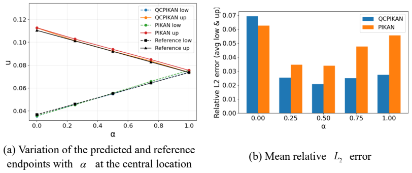
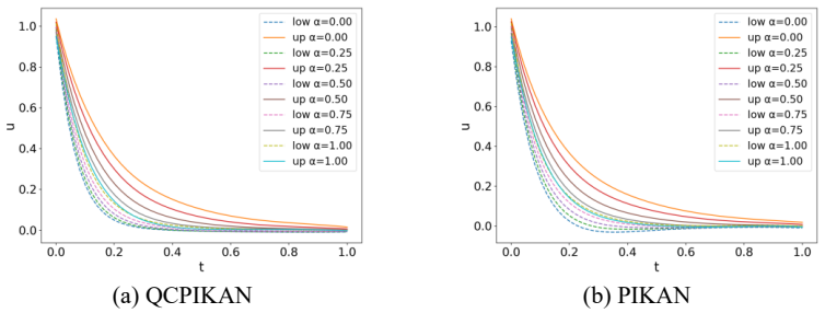
The central claim is that a single network in which classical ChebyKAN layers sandwich a parameterized quantum circuit can jointly approximate the lower and upper $\alpha$-cut endpoint functions of a fuzzy PDE solution, and that this hybrid representation can be more accurate than the classical PIKAN baseline. Theorem 1 decomposes the endpoint-solution error of each model into approximation, optimization, finite-sampling, fuzzy-structure, gradient, and hardware-noise components and shows that QCPIKAN has a strictly smaller a priori bound exactly when its representation gain $\Delta^{\mathrm{app}}$ dominates the sum of the extra computational errors. Under the ideal-simulation conditions used, this condition reduces to comparing the representation gain with the optimization, sampling, and structure-constraint error differences. Numerical experiments on a fuzzy Poisson equation, a fuzzy heat-conduction equation, a fuzzy reaction-diffusion equation, and a fuzzy convection equation support the claimed advantage: PIKAN's mean relative $L^2$ errors are about 1.1--2.7 times QCPIKAN's at most membership levels, and its mean wavefront-position error is about 1.77 times larger, while both models retain local endpoint-ordering and nesting violations near boundaries, high gradients, and the wavefront.
Load-bearing premise
The argument stands or falls on the assumption that, at a fixed model size, the QCPIKAN feature space can reproduce or beat the classical PIKAN representation on the nonseparable part of the fuzzy solution; the paper assumes this representation gain (A3) rather than measuring it independently of the experiments it is used to explain.
Editorial extensions
If this is right
- One trained QCPIKAN returns the entire nested family of $\alpha$-cut interval solutions, with $\alpha$ as a continuous input, for elliptic, parabolic, and hyperbolic fuzzy PDEs.
- On the four test equations, PIKAN's mean relative $L^2$ error is about 1.1--2.7 times QCPIKAN's at most tested membership levels, and its mean wavefront-position error in the convection example is about 1.77 times larger.
- The theoretical comparison is conditional: QCPIKAN beats PIKAN only when the representation gain from the quantum feature space exceeds the combined extra optimization, sampling, fuzzy-structure, gradient, and hardware errors, so the advantage is not automatic.
- Both models still violate fuzzy-structure constraints locally near boundaries, in high-gradient regions, and around the wavefront, so soft penalty enforcement does not guarantee a globally valid fuzzy solution.
- Within the tested range, QCPIKAN accuracy improves with qubit count but varies nonmonotonically with circuit depth, consistent with growing optimization difficulty, including barren-plateau effects, at larger depth.
Reading between the lines
- A direct extension not tested in the paper: the same ChebyKAN-plus-quantum-circuit architecture could serve as a general solver for parametric families of PDEs whose solutions depend nonseparably on the parameters, not only on the fuzzy membership level.
- Because both models retain fuzzy-structure violations despite soft penalties, a natural next experiment is to enforce endpoint ordering and inter-level nesting with hard architectural constraints, such as monotonic output layers, to test whether the residual violations are a representation issue or a training issue.
- The numerical comparisons use an ideal quantum simulator with analytic expectation values; on real hardware the finite-shot and gate-noise terms in Eq. (43) would enter, so the practical advantage should be re-measured under finite-shot conditions before drawing hardware conclusions.
- To attribute the lower errors to quantum entanglement features, one would need a matched classical counterfactual with interaction features at the same parameter count, since the paper does not isolate $\Delta^{\mathrm{app}}$ independently of the experiments.
Signed reviews
Editorial analysis
A structured set of objections, weighed in public.
Referee Report
Summary. The manuscript proposes QCPIKAN, a hybrid classical-quantum architecture that combines ChebyKAN layers with a four-qubit parameterized quantum circuit to solve fuzzy partial differential equations represented through alpha-cuts. The model treats the spatiotemporal coordinates and the membership level as joint inputs and outputs the lower and upper alpha-cut endpoint functions simultaneously. Its loss function includes the endpoint governing equations, initial and boundary conditions, endpoint ordering, inter-level nesting, and endpoint coincidence at alpha = 1. Section 2.3 presents an error decomposition and Theorem 1, which states that QCPIKAN has a smaller a priori error bound than PIKAN when the representation gain Delta_app exceeds the sum of the remaining computational-error differences. Numerical experiments cover a fuzzy Poisson equation, a fuzzy heat-conduction equation, a fuzzy reaction-diffusion equation, and a fuzzy convection equation, reporting that PIKAN's mean relative L2 error is approximately 1.1-2.7 times larger at most tested membership levels and that the wavefront-position error is about 1.77 times larger on average. The manuscript is candid that both models still exhibit local fuzzy-structure violations and that the experiments use an ideal quantum simulator.
Significance. If the central claims were established, the paper would offer a useful computational framework for fuzzy PDEs that integrates KAN-based function representation, variational quantum circuits, and explicit fuzzy-structure constraints in a single physics-informed objective. The four numerical examples cover elliptic, parabolic, and hyperbolic problems, and the error metrics include both endpoint L2 errors and a wavefront-position error, which are appropriate for the considered problems. The paper also deserves credit for explicitly separating representation, optimization, sampling, fuzzy-structure, gradient, and hardware-noise errors, and for acknowledging that neither model strictly satisfies the fuzzy-structure constraints. However, the advertised theoretical result is essentially a restatement of its assumption, and the numerical experiments do not isolate the effect of the quantum feature map from additional classical capacity. As presented, the contribution is a plausible architecture plus a single-run numerical comparison whose central quantum-advantage claim is not yet established.
major comments (3)
- [Sec. 2.3, Theorem 1, Eqs. (43)-(45)] The theorem's sufficient condition is algebraically identical to its conclusion. Substituting Delta_app = E_app^P - E_app^Q into Eq. (43) gives E_app^Q + eps_Q < E_app^P + eps_P, and multiplying by C_stab yields exactly the claimed bound inequality Eq. (45). Thus Theorem 1 does not establish any nontrivial condition under which QCPIKAN beats PIKAN; it merely restates the target inequality after assuming, through Assumption A3, that QCPIKAN's best-approximation error is sufficiently smaller. The paper provides no independent estimate or bound for Delta_app, and the numerical experiments used to verify Eq. (44) are the same experiments that would need to supply Delta_app. Please reframe the theorem as an error decomposition with a stated condition, or provide an independent argument that Delta_app is positive and sufficiently large for the considered architecture.
- [Sec. 3 and Sec. 2.2.2] The empirical comparison does not isolate the quantum feature map from classical model capacity. The QCPIKAN pipeline is described as ChebyKAN 3->30->4, followed by a four-qubit circuit, followed by ChebyKAN 4->30->2, but the PIKAN architecture, its width, depth, and total parameter count are never specified. The reported 1.1-2.7x error ratios could therefore be caused by the extra ChebyKAN width, depth, or optimization capacity rather than by the entanglement features of the circuit. The paper should specify the PIKAN architecture exactly and include a counterfactual ablation in which the quantum circuit is replaced by a classical trainable nonlinear mixing layer of identical parameter count and comparable capacity.
- [Sec. 3, general experimental protocol] All numerical results appear to be single-run experiments without reported seeds, repeated trials, confidence intervals, or code. Because the reported performance ratios are as small as 1.1x, it is not possible to assess whether the observed differences are statistically meaningful or robust to initialization. The paper should report multi-seed statistics, specify all sampling sizes, and ideally provide code to make the comparison reproducible. This is load-bearing for the central empirical claim that PIKAN's mean relative L2 error is 1.1-2.7 times that of QCPIKAN.
minor comments (5)
- [Sec. 3.1] The text says QCPIKAN and PIKAN approximate Lu_alpha and Uu_alpha 'in Eq. (36)', but Eq. (36) is the generic error-bound inequality; the intended reference appears to be Eq. (51).
- [Eq. (52)] The Fourier sine-series reference solution contains garbled notation, including an apparent '?' character and an unclear summation range 'm,n odd, 1<=m,n<=49'. Please clean up the displayed formula and define all summation limits clearly.
- [Example 4, Eq. (60)] The initial condition for the convection equation is garbled in the displayed equation; the intended condition appears to be u(x,0)=u_0(x), but it should be written out explicitly.
- [Secs. 3.3 and 3.4] The manuscript honestly reports that in Example 3 QCPIKAN has more widely distributed inter-level nesting violations than PIKAN and that in Example 4 it does not show a consistent advantage in fuzzy-structure metrics. Since fuzzy-structure satisfaction is part of the model's stated objective, the paper should present quantitative structure-violation statistics and temper the conclusion that QCPIKAN provides a more accurate fuzzy solution family.
- [Sec. 2.2.3] The loss weights are chosen separately for each example and are not subjected to sensitivity analysis. A brief study of how the reported error ratios vary with these weights would strengthen the numerical comparison.
Circularity Check
Theorem 1's conclusion is a restatement of its main assumption: Eq. (43) is algebraically identical to Eq. (45), and the experiments cited as 'verification of Eq. (44)' never isolate the quantum feature-map advantage.
-
self definitional
[Sec. 2.3, Theorem 1 and proof, Eqs. (41)-(48)]
"Second, Eq. (43) is equivalent to (E_Q^app + ε_Q) - (E_P^app + ε_P) < 0. ... Because the stability constant C_stab > 0, multiplying both sides of Eq. (47) by C_stab does not change the direction of the inequality. Therefore, C_stab(E_Q^app + ε_Q) < C_stab(E_P^app + ε_P). Thus, E_Q < E_P and Eq. (45) holds, completing the proof."
Two paragraphs earlier the paper defines Δ_app = E_P^app − E_Q^app (Eq. (41)). Substituting that definition into condition (43) yields exactly E_Q^app + ε_Q < E_P^app + ε_P, which is Eq. (47). Multiplying by C_stab produces E_Q < E_P, the theorem's conclusion. So Theorem 1 does not derive the quantum advantage from independent premises; it restates, in decomposed notation, the assumption that QCPIKAN's approximation advantage outweighs its computational-error disadvantage. Assumption A3 already assumes a strict best-approximation advantage at fixed model size, and no independent estimate of Δ_app is supplied.
-
fitted input called prediction
[Sec. 2.3, final paragraph; Sec. 3 numerical experiments]
"The numerical results presented here should therefore be interpreted as empirical verification of Eq. (44) under ideal conditions."
Eq. (44) is the theorem's sufficient-condition inequality, which is algebraically equivalent to the claimed bound comparison E_Q < E_P. The experiments report final mean relative L2 errors, wavefront-position errors, and loss curves — the same quantities the bound comparison concerns — but never measure E_Q^app, E_P^app, or the individual optimization, sampling, and fuzzy-structure error terms at a fixed PIKAN parameter count. PIKAN's architecture and total parameter count are not specified, and QCPIKAN adds ChebyKAN layers 3→30→4 before and 4→30→2 after the circuit. Thus 'empirical verification of Eq.
full rationale
The paper contains no load-bearing self-citation: [65] and [66] are contextual references, and the fuzzy-structure losses and ChebyKAN-plus-circuit architecture are described directly. The numerical benchmarks are also self-contained against analytic eigenfunction series, exact heat-kernel solutions, IMEX finite differences, and method-of-characteristics solutions, so the empirical comparisons have independent content. The central theoretical result, however, is tautological. With Δ_app defined as E_P^app − E_Q^app, inequality (43) is exactly E_Q^app + ε_Q < E_P^app + ε_P; multiplying by C_stab gives E_Q < E_P, the theorem's conclusion. Assumption A3 already assumes the strict approximation advantage, and the paper offers no independent estimate of Δ_app. The experiments do not close this gap: PIKAN's architecture and parameter count are unspecified, and QCPIKAN's extra ChebyKAN layers precede and follow the quantum circuit, so the observed 1.1–2.7x error ratios cannot be uniquely attributed to quantum entanglement features. Calling the numerical results 'verification of Eq. (44)' is circular in the sense that Eq. (44) is the same algebraic comparison as the claimed bound advantage. Overall, the error decomposition and benchmarks have independent value, but the advertised a priori quantum-advantage theorem reduces by construction to its own assumption, giving a partial-circularity score of 5.
Assumptions & free parameters
free parameters (5)
- Loss weights, Example 1 (lambda_res, lambda_BC, lambda_nest, lambda_order, lambda_{alpha=1}) =
1, 1, 0.1, 0.2, 1
- Loss weights, Example 2 (lambda_res, lambda_IC, lambda_BC, lambda_nest, lambda_order, lambda_{alpha=1}) =
1, 1, 1, 0.5, 0.2, 1
- Loss weights, Example 3 (lambda_res, lambda_IC, lambda_BC, lambda_nest, lambda_order, lambda_{alpha=1}) =
1, 1, 1, 0.1, 0.2, 1
- Loss weights, Example 4 (lambda_res, lambda_IC, lambda_BC, lambda_nest, lambda_order, lambda_{alpha=1}) =
5, 10, 5, 0.5, 0.15, 0.15
- Qubit count and circuit depth =
n_q = 4, 1 variational layer
assumptions (5)
- domain assumption Residual-stability estimate Eq. (35): ||U - V||_H <= C_stab ||R(V) - R(U)||_Y
- domain assumption Endpoint problems are well-posed (A1)
- domain assumption Monotonic dependence of solution endpoints on fuzzy parameters in Examples 2-4 (e.g., Eq. (55) uses a_U for the lower endpoint, Eq. (59) uses (a_U, b_L), Eq. (62) uses c_U)
- domain assumption Ideal quantum simulation with analytic expectation values and no noise
- standard math Triangular fuzzy inputs with singleton core imply endpoint coincidence at alpha = 1 (Eq. (9))
Cite this review
Pith. "Pith review of Quantum-Classical Physics-Informed Kolmogorov-Arnold Networks for Solving Fuzzy Differential Equations." pith.science (2026). https://pith.science/paper/47CESTSD
@misc{pith2026260808782,
  author       = {Pith},
  title        = {Pith review of: Quantum-Classical Physics-Informed Kolmogorov-Arnold Networks for Solving Fuzzy Differential Equations},
  year         = {2026},
  howpublished = {\url{https://pith.science/paper/47CESTSD}},
  note         = {Machine review of arXiv:2608.08782}
}
read the original abstract
In this study, we propose a quantum-classical physics-informed Kolmogorov-Arnold network (QCPIKAN) dedicated to the solution of fuzzy differential equations. The network takes the spatiotemporal coordinates and membership level as joint inputs and employs ChebyKAN modules and a parameterized quantum circuit to construct a hybrid function approximator. It simultaneously approximates the lower and upper endpoint functions associated with the {\alpha}-cuts and incorporates the governing equations, initial-boundary conditions, and fuzzy-structural constraints into the training objective. Theoretically, a unified error-analysis framework is established for QCPIKAN and PIKAN, in which the endpoint-solution error is decomposed into approximation, sampling, optimization, and fuzzy-structure constraint errors. Under the assumptions of well-posedness and residual stability, it is proved that QCPIKAN has a smaller a priori error bound when the representational gain introduced by quantum entanglement features exceeds the additional computational error. Numerical experiments are conducted for elliptic, parabolic, and hyperbolic equations in an ideal quantum-simulation environment. The results show that QCPIKAN captures the overall contraction of the solution interval as increases. At most tested membership levels, the mean relative L2 error of PIKAN is approximately 1.1-2.7 times that of QCPIKAN. In the fuzzy convection example, the mean wavefront-position error of PIKAN is approximately 1.77 times that of QCPIKAN. Nevertheless, both models still exhibit local fuzzy-structure violations near boundaries, in high-gradient regions, and around the wavefront. These results indicate that QCPIKAN provides a quantum-classical hybrid physics-informed computational framework with comparatively high predictive accuracy for solving fuzzy partial differential equations represented by {\alpha}-cuts.
Figures



Figures from the paper (18 more)






Reference graph
Works this paper leans on
-
[30]
Interval and fuzzy physics -informed neural networks for uncertain fields,
J. N. Fuhg, I. Kalogeris, A. Fau, and N. Bouklas, “Interval and fuzzy physics -informed neural networks for uncertain fields,” Probabilistic Engineering Mechanics , vol. 68, p. 103240, Apr. 2022, doi: 10.1016/j.probengmech.2022.103240
arXiv 2022
-
[41]
A. Kazemi, A. A. Aghaei, and A. Nazemi, “Physics -informed kolmogorov -arnold networks for granular fuzzy fractional optimal control problems,” IEEE Trans. Fuzzy Syst., pp. 1–10, 2026, doi: 10.1109/TFUZZ.2026.3698597
-
[1]
L. A. Zadeh, “Fuzzy sets,” Information and Control, vol. 8, no. 3, pp. 338–353, Jun. 1965, doi: 10.1016/S0019-9958(65)90241-X
-
[2]
Introduction to fuzzy partial differential equations,
J. J. Buckley and T. Feuring, “Introduction to fuzzy partial differential equations,” Fuzzy Sets and Systems , vol. 105, no. 2, pp. 241 –248, Jul. 1999, doi: 10.1016/S0165 - 0114(98)00323-6
-
[3]
Z. Gouyandeh, T. Allahviranloo, S. Abbasbandy, and A. Armand, “A fuzzy solution of heat equation under generalized hukuhara differentiability by fuzzy fourier transform,” Fuzzy Sets and Systems, vol. 309, pp. 81–97, Feb. 2017, doi: 10.1016/j.fss.2016.04.010
-
[4]
Solving fuzzy burgers equation by variational iteration method,
A. Harir, S. Melliani, and L. Saadia Chadli, “Solving fuzzy burgers equation by variational iteration method,” J. Math. Computer Sci., vol. 21, no. 02, pp. 136–149, Apr. 2020, doi: 10.22436/jmcs.021.02.05
-
[5]
A. Pownuk, “Numerical solutions of fuzzy partial differential equations and its applications in computational mechanics,” in Fuzzy Partial Differential Equations and Relational Equations, vol. 142, M. Nikravesh, L. A. Zadeh, and V . Korotkikh, Eds., in Studies in Fuzziness and Soft Computing, vol. 142. , Berlin, Heidelberg: Springer Berlin Heidelberg, 200...
-
[6]
R. Goetschel and W. V oxman, “Elementary fuzzy calculus,” Fuzzy Sets and Systems, vol. 18, no. 1, pp. 31–43, Jan. 1986, doi: 10.1016/0165-0114(86)90026-6
Show all 67 references
-
[7]
Parametric representation of fuzzy numbers and application to fuzzy calculus,
L. Stefanini, L. Sorini, and M. L. Guerra, “Parametric representation of fuzzy numbers and application to fuzzy calculus,” Fuzzy Sets and Systems, vol. 157, no. 18, pp. 2423 – 2455, Sep. 2006, doi: 10.1016/j.fss.2006.02.002
2006 doi
-
[8]
On using α-cuts to evaluate fuzzy equations,
J. J. Buckley and Y . Qu, “On using α-cuts to evaluate fuzzy equations,” Fuzzy Sets and Systems, vol. 38, no. 3, pp. 309–312, Dec. 1990, doi: 10.1016/0165-0114(90)90204-J
1990 doi
-
[9]
Zadeh’s extension principle for continuous functions of non -interactive variables: A parallel optimization approach,
K. Scheerlinck, H. Vernieuwe, and B. De Baets, “Zadeh’s extension principle for continuous functions of non -interactive variables: A parallel optimization approach,” IEEE Trans. Fuzzy Syst. , vol. 20, no. 1, pp. 96 –108, Feb. 2012, doi : 10.1109/TFUZZ.2011.2168406
2012
-
[10]
Difference methods for fuzzy partial differential equations,
T. Allahviranloo, “Difference methods for fuzzy partial differential equations,” Comput. Methods Appl. Math., vol. 2, no. 3, pp. 233–242, 2002, doi: 10.2478/cmam-2002-0014
2002 doi
-
[11]
Neural‐network‐based approximations for solving partial differential equations,
M. W. M. G. Dissanayake and N. Phan‐Thien, “Neural‐network‐based approximations for solving partial differential equations,” Commun. Numer. Meth. Engng., vol. 10, no. 3, pp. 195–201, Mar. 1994, doi: 10.1002/cnm.1640100303
1994 doi
-
[12]
Artificial neural networks for solving ordinary and partial differential equations,
I. E. Lagaris, A. Likas, and D. I. Fotiadis, “Artificial neural networks for solving ordinary and partial differential equations,” IEEE Trans. Neural Netw., vol. 9, no. 5, pp. 987–1000, Sep. 1998, doi: 10.1109/72.712178
1998 doi
-
[13]
Physics -informed neural networks: A deep learning framework for solving forward and inverse problems involving nonlinear partial differential equations,
M. Raissi, P. Perdikaris, and G. E. Karniadakis, “Physics -informed neural networks: A deep learning framework for solving forward and inverse problems involving nonlinear partial differential equations,” Journal of Computational Physics, vol. 378, pp. 686–707, Feb. 2019, doi:...
2019 doi
-
[14]
Physics- informed machine learning,
G. E. Karniadakis, I. G. Kevrekidis, L. Lu, P. Perdikaris, S. Wang, and L. Yang, “Physics- informed machine learning,” Nat Rev Phys, vol. 3, no. 6, pp. 422 –440, May 2021, doi: 10.1038/s42254-021-00314-5
2021 doi
-
[15]
Physics-informed neural networks for inverse problems in nano -optics and metamaterials,
Y . Chen, L. Lu, G. E. Karniadakis, and L. Dal Negro, “Physics-informed neural networks for inverse problems in nano -optics and metamaterials,” Opt. Express, vol. 28, no. 8, p. 11618, Apr. 2020, doi: 10.1364/OE.384875
2020 doi
-
[16]
Physics-informed neural networks for cardiac activation mapping,
F. Sahli Costabal, Y . Yang, P. Perdikaris, D. E. Hurtado, and E. Kuhl, “Physics-informed neural networks for cardiac activation mapping,” Front. Phys., vol. 8, p. 42, Feb. 2020, doi: 10.3389/fphy.2020.00042
2020
-
[17]
A physics-informed deep learning framework for inversion and surrogate modeling in solid mechanics,
E. Haghighat, M. Raissi, A. Moure, H. Gomez, and R. Juanes, “A physics-informed deep learning framework for inversion and surrogate modeling in solid mechanics,” Computer Methods in Applied Mechanics and Engineering , vol. 379, p. 113741, Jun. 2021, doi: 10.1016/j.cma.2021.113741
2021
-
[18]
AI -aristotle: A physics -informed framework for systems biology gray -box identification,
N. Ahmadi Daryakenari, M. De Florio, K. Shukla, and G. E. Karniadakis, “AI -aristotle: A physics -informed framework for systems biology gray -box identification,” PLoS Comput Biol, vol. 20, no. 3, p. e1011916, Mar. 2024, doi: 10.1371/journal.pcbi.1011916
2024 doi
-
[19]
Physics-informed neural network (PINN) for solving frictional contact temperature and inversely evaluating relevant input parameters,
Y . Xia and Y . Meng, “Physics-informed neural network (PINN) for solving frictional contact temperature and inversely evaluating relevant input parameters,” Lubricants, vol. 12, no. 2, p. 62, Feb. 2024, doi: 10.3390/lubricants12020062
2024 doi
-
[20]
Physics‐informed deep neural networks for learning parameters and constitutive relationships in subsurface flow problems,
A. M. Tartakovsky, C. O. Marrero, P. Perdikaris, G. D. Tartakovsky, and D. Barajas‐ Solano, “Physics‐informed deep neural networks for learning parameters and constitutive relationships in subsurface flow problems,” Water Resources Research, vol. 56, no. 5, p. e2019WR026731, M...
2020 doi
-
[21]
Physics -informed neural networks with weighted losses by uncertainty evaluation for accurate and stable prediction of manufacturing systems,
J. Hua, Y . Li, C. Liu, P. Wan, and X. Liu, “Physics -informed neural networks with weighted losses by uncertainty evaluation for accurate and stable prediction of manufacturing systems,” IEEE Trans. Neural Netw. Learning Syst. , vol. 35, no. 8, pp. 11064–11076, Aug. 2024, doi...
2024
-
[22]
Residual- based adaptivity for two-phase flow simulation in porous media using physics-informed neural networks,
J. M. Hanna, J. V . Aguado, S. Comas-Cardona, R. Askri, and D. Borzacchiello, “Residual- based adaptivity for two-phase flow simulation in porous media using physics-informed neural networks,” Computer Methods in Applied Mechanics and Engineering , vol. 396, p. 115100, Jun. 20...
2022
-
[23]
Weak form theory -guided neural network (TgNN-wf) for deep learning of subsurface single - and two -phase flow,
R. Xu, D. Zhang, M. Rong, and N. Wang, “Weak form theory -guided neural network (TgNN-wf) for deep learning of subsurface single - and two -phase flow,” Journal of Computational Physics, vol. 436, p. 110318, Jul. 2021, doi: 10.1016/j.jcp.2021.110318
2021
-
[24]
A mixed pressure-velocity formulation to model flow in heterogeneous porous media with physics -informed neural networks,
F. Lehmann, M. Fahs, A. Alhubail, and H. Hoteit, “A mixed pressure-velocity formulation to model flow in heterogeneous porous media with physics -informed neural networks,” Advances in Water Resources , vol. 181, p. 104564, Nov. 2023, doi : 10.1016/j.advwatres.2023.104564
2023
-
[25]
Physics -informed hybrid GRU neural networks for MPC prediction,
K. Zarzycki and M. Lawryńczuk, “Physics -informed hybrid GRU neural networks for MPC prediction,” IFAC-PapersOnLine, vol. 56, no. 2, pp. 8726 –8731, 2023, doi: 10.1016/j.ifacol.2023.10.055
2023 doi
-
[26]
Physics -informed spatial fuzzy system and its applications in modeling,
H.-P. Deng, B.-C. Wang, and H.-X. Li, “Physics -informed spatial fuzzy system and its applications in modeling,” IEEE Trans. Fuzzy Syst., vol. 32, no. 10, pp. 5951–5962, Oct. 2024, doi: 10.1109/TFUZZ.2024.3439537
2024
-
[27]
Deep fuzzy physics-informed neural networks for forward and inverse PDE problems,
W. Wu, S. Duan, Y . Sun, Y . Yu, D. Liu, and D. Peng, “Deep fuzzy physics-informed neural networks for forward and inverse PDE problems,” Neural Networks, vol. 181, p. 106750, Jan. 2025, doi: 10.1016/j.neunet.2024.106750
2025
-
[28]
On physics-informed fuzzy neural network for the state of health prediction of lithium-ion batteries,
Z. Ren and Y . Wei, “On physics-informed fuzzy neural network for the state of health prediction of lithium-ion batteries,” Journal of Energy Storage, vol. 155, p. 121467, Apr. 2026, doi: 10.1016/j.est.2026.121467
2026
-
[29]
Physics -informed neural network with fuzzy partial differential equation for pavement performance prediction,
J. Li, S. Zhang, and X. Wang, “Physics -informed neural network with fuzzy partial differential equation for pavement performance prediction,” Automation in Construction, vol. 171, p. 105983, Mar. 2025, doi: 10.1016/j.autcon.2025.105983
2025
-
[31]
Understanding and Mitigating Gradient Flow Pathologies in Physics-Informed Neural Networks,
S. Wang, Y . Teng, and P. Perdikaris, “Understanding and Mitigating Gradient Flow Pathologies in Physics-Informed Neural Networks,” SIAM J. Sci. Comput., vol. 43, no. 5, pp. A3055–A3081, Jan. 2021, doi: 10.1137/20M1318043
2021 doi
-
[32]
When and why PINNs fail to train: A neural tangent kernel perspective,
S. Wang, X. Yu, and P. Perdikaris, “When and why PINNs fail to train: A neural tangent kernel perspective,” Journal of Computational Physics , vol. 449, p. 110768, Jan. 2022, doi: 10.1016/j.jcp.2021.110768
2022
-
[33]
Boundary-integral type neural network (BINN) for flow problems in anisotropic reservoirs,
X. Rao et al. , “Boundary-integral type neural network (BINN) for flow problems in anisotropic reservoirs,” in Middle East Oil, Gas and Geosciences Show (MEOS GEO) , Manama, Bahrain: SPE, Sep. 2025, p. D021S048R001. doi: 10.2118/227536-MS
2025 doi
- [34]
-
[35]
A comprehensive and FAIR comparison between MLP and KAN representations for differential equations and operator networks,
K. Shukla, J. D. Toscano, Z. Wang, Z. Zou, and G. E. Karniadakis, “A comprehensive and FAIR comparison between MLP and KAN representations for differential equations and operator networks,” Computer Methods in Applied Mechanics and Engineering, vol. 431, p. 117290, Nov. 2024, ...
2024
-
[36]
Physics -informed kolmogorov-arnold networks for power system dynamics,
H. Shuai and F. Li, “Physics -informed kolmogorov-arnold networks for power system dynamics,” IEEE Open J. Power Energy , vol. 12, pp. 46 –58, 2025, doi: 10.1109/OAJPE.2025.3529928
2025
-
[37]
Physics -informed KAN-coupled FEM for deformation analysis of complex shells,
M.-Z. Huang, Y .-X. Peng, Z. -T. Jiang, P.-N. Sun, and C. -X. Jiang, “Physics -informed KAN-coupled FEM for deformation analysis of complex shells,” Thin-Walled Structures, vol. 216, p. 113725, Nov. 2025, doi: 10.1016/j.tws.2025.113725
2025
-
[38]
Physics-informed kolmogorov–arnold networks to model flow in heterogeneous porous media with a mixed pressure-velocity formulation,
X. Rao, Y . Liu, X. He, and H. Hoteit, “Physics-informed kolmogorov–arnold networks to model flow in heterogeneous porous media with a mixed pressure-velocity formulation,” Physics of Fluids, vol. 37, no. 7, p. 076654, Jul. 2025, doi: 10.1063/5.0279122
2025 doi
-
[39]
Physics -informed kolmogorov-arnold networks for multi -material elasticity problems in electronic packaging,
Y . Gong, Y . He, Y . Mei, X. Zhuang, F. Qin, and T. Rabczuk, “Physics -informed kolmogorov-arnold networks for multi -material elasticity problems in electronic packaging,” Applied Mathematical Modelling , vol. 156, p. 116793, Aug. 2026, doi: 10.1016/j.apm.2026.116793
2026
-
[40]
Parameterized analytical solution of seepage equation for reservoir simulation using physics -informed kolmogorov -arnold network without labels,
Q. Wang, W. Zha, D. Li, X. Li, L. Shen, and Z. Shi, “Parameterized analytical solution of seepage equation for reservoir simulation using physics -informed kolmogorov -arnold network without labels,” Journal of Computational Physics , vol. 548, p. 114599, Mar. 2026, doi: 10.10...
2026
-
[42]
Quantum computing in the NISQ era and beyond,
J. Preskill, “Quantum computing in the NISQ era and beyond,” Quantum, vol. 2, p. 79, Aug. 2018, doi: 10.22331/q-2018-08-06-79
2018 doi
-
[43]
Noisy intermediate-scale quantum algorithms,
K. Bharti et al., “Noisy intermediate-scale quantum algorithms,” Rev. Mod. Phys., vol. 94, no. 1, p. 015004, Feb. 2022, doi: 10.1103/RevModPhys.94.015004
2022 doi
-
[44]
Performance study of variational quantum linear solver with an improved ansatz for reservoir flow equations,
X. Rao, “Performance study of variational quantum linear solver with an improved ansatz for reservoir flow equations,” Physics of Fluids, vol. 36, no. 4, p. 047104, Apr. 2024, doi: 10.1063/5.0201739
2024 doi
-
[45]
Performance study of variational quantum linear solver for linear elastic problems,
X. Rao and K. Du, “Performance study of variational quantum linear solver for linear elastic problems,” in Computational and Experimental Simulations in Engineering, vol. 168, K. Zhou, Ed., in Mechanisms and Machine Science, vol. 168. , Cham: Springer Nature Switzerland, 2024,...
2024 doi
-
[46]
Data re -uploading for a universal quantum classifier,
A. Pérez-Salinas, A. Cervera-Lierta, E. Gil-Fuster, and J. I. Latorre, “Data re -uploading for a universal quantum classifier,” Quantum, vol. 4, p. 226, Feb. 2020, doi: 10.22331/q- 2020-02-06-226
2020 doi
-
[47]
Universal Approximation Theorem and Error Bounds for Quantum Neural Networks and Quantum Reservoirs,
L. Gonon and A. Jacquier, “Universal Approximation Theorem and Error Bounds for Quantum Neural Networks and Quantum Reservoirs,” IEEE Trans. Neural Netw. Learning Syst. , vol. 36, no. 6, pp. 11355 –11368, Jun. 2025, doi: 10.1109/TNNLS.2025.3552223
2025
-
[48]
The power of quantum neural networks,
A. Abbas, D. Sutter, C. Zoufal, A. Lucchi, A. Figalli, and S. Woerner, “The power of quantum neural networks,” Nat Comput Sci, vol. 1, no. 6, pp. 403 –409, Jun. 2021, doi: 10.1038/s43588-021-00084-1
2021 doi
-
[49]
Supervised learning with quantum-enhanced feature spaces,
V . Havlíček et al., “Supervised learning with quantum-enhanced feature spaces,” Nature, vol. 567, no. 7747, pp. 209–212, Mar. 2019, doi: 10.1038/s41586-019-0980-2
2019 doi
-
[50]
A quantum spatial graph convolutional neural network model on quantum circuits,
J. Zheng, Q. Gao, M. Ogorza łek, J. Lü, and Y . Deng, “A quantum spatial graph convolutional neural network model on quantum circuits,” IEEE Trans. Neural Netw. Learning Syst. , vol. 36, no. 3, pp. 5706 –5720, Mar. 2025, doi: 10.1109/TNNLS.2024.3382174
2025
-
[51]
Solving nonlinear differential equations with differentiable quantum circuits,
O. Kyriienko, A. E. Paine, and V . E. Elfving, “Solving nonlinear differential equations with differentiable quantum circuits,” Phys. Rev. A, vol. 103, no. 5, p. 052416, May 2021, doi: 10.1103/PhysRevA.103.052416
2021 doi
-
[52]
An efficient quantum neural network model for prediction of carbon dioxide CO2 sequestration in saline aquifers,
X. Rao, C. Luo, X. He, and K. Hyung, “An efficient quantum neural network model for prediction of carbon dioxide CO2 sequestration in saline aquifers,” in ADIPEC, Abu Dhabi, UAE: SPE, Nov. 2024, p. D021S061R005. doi: 10.2118/222257-MS
2024 doi
-
[53]
Barren plateaus in quantum neural network training landscapes,
J. R. McClean, S. Boixo, V . N. Smelyanskiy, R. Babbush, and H. Neven, “Barren plateaus in quantum neural network training landscapes,” Nat Commun, vol. 9, no. 1, p. 4812, Nov. 2018, doi: 10.1038/s41467-018-07090-4
2018 doi
-
[54]
Noise-induced barren plateaus in variational quantum algorithms,
S. Wang et al., “Noise-induced barren plateaus in variational quantum algorithms,” Nat Commun, vol. 12, no. 1, p. 6961, Nov. 2021, doi: 10.1038/s41467-021-27045-6
2021 doi
-
[55]
On physics-informed neural networks for quantum computers,
S. Markidis, “On physics-informed neural networks for quantum computers,” Front. Appl. Math. Stat., vol. 8, p. 1036711, Oct. 2022, doi: 10.3389/fams.2022.1036711
2022
-
[56]
Quantum physics -informed neural networks,
C. Trahan, M. Loveland, and S. Dent, “Quantum physics -informed neural networks,” Entropy, vol. 26, no. 8, p. 649, Jul. 2024, doi: 10.3390/e26080649
2024 doi
-
[57]
Physics-informed quantum neural network for solving forward and inverse problems of partial differential equations,
Y . Xiao et al., “Physics-informed quantum neural network for solving forward and inverse problems of partial differential equations,” Physics of Fluids, vol. 36, no. 9, p. 097145, Sep. 2024, doi: 10.1063/5.0226232
2024 doi
-
[58]
Trainable embedding quantum physics informed neural networks for solving nonlinear PDEs,
S. Berger, N. Hosters, and M. Möller, “Trainable embedding quantum physics informed neural networks for solving nonlinear PDEs,” Sci Rep, vol. 15, no. 1, p. 18823, May 2025, doi: 10.1038/s41598-025-02959-z
2025 doi
-
[59]
Quantum physics -informed neural networks for multivariable partial differential equations,
G. Panichi, S. Corli, and E. Prati, “Quantum physics -informed neural networks for multivariable partial differential equations,” Phys. Rev. Applied, vol. 25, no. 1, p. 014001, Jan. 2026, doi: 10.1103/6nh4-yh2y
2026 doi
-
[60]
Exploring hybrid physics - informed neural networks with quantum layers for solving the wave equation,
B. O. Fernandez, C. Leao, D. E. Revelo, and G. Fernandes, “Exploring hybrid physics - informed neural networks with quantum layers for solving the wave equation,” in Fifth EAGE Digitalization Conference & Exhibition, Edinburgh, Scotland, United Kingdom,: European Association o...
2025
-
[61]
QCPINN: Quantum -classical physics - informed neural networks for solving PDEs,
A. Farea, S. Khan, and M. Serdar Celebi, “QCPINN: Quantum -classical physics - informed neural networks for solving PDEs,” Mach. Learn.: Sci. Technol., vol. 6, no. 4, p. 045053, Dec. 2025, doi: 10.1088/2632-2153/ae1c91
2025 doi
-
[62]
Hybrid quantum physics-informed neural network: Towards efficient learning of high -speed flows,
F. Y . Leong, W.-B. Ewe, S. B. Q. Tran, Z. Zhang, and J. Y . Khoo, “Hybrid quantum physics-informed neural network: Towards efficient learning of high -speed flows,” Computers & Fluids , vol. 301, p. 106782, Oct. 2025, doi: 10.1016/j.compfluid.2025.106782
2025
-
[63]
Incompressible navier–stokes solve on noisy quantum hardware via a hybrid quantum –classical scheme,
Z. Song, R. Deaton, B. Gard, and S. H. Bryngelson, “Incompressible navier–stokes solve on noisy quantum hardware via a hybrid quantum –classical scheme,” Computers & Fluids, vol. 288, p. 106507, Feb. 2025, doi: 10.1016/j.compfluid.2024.106507
2025
-
[64]
A hybrid quantum-classical physics- informed neural network architecture for solving quantum optimal control problems,
N. B. Dehaghani, A. P. Aguiar, and R. Wisniewski, “A hybrid quantum-classical physics- informed neural network architecture for solving quantum optimal control problems,” 2024, arXiv. doi: 10.48550/ARXIV .2404.15015
-
[65]
Quantum-classical physics-informed neural networks for solving reservoir seepage equations,
X. Rao, Y . Liu, and Y . Shen, “Quantum-classical physics-informed neural networks for solving reservoir seepage equations,” 2025, arXiv. doi: 10.48550/ARXIV .2512.03923
2025 doi
- [66]
-
[67]
Chebyshev polynomial -based kolmogorov -arnold networks: An efficient architecture for nonlinear function approximation,
S. SS, K. AR, G. R, and A. KP, “Chebyshev polynomial -based kolmogorov -arnold networks: An efficient architecture for nonlinear function approximation,” 2024, arXiv. doi: 10.48550/ARXIV .2405.07200
Reviewed August 14, 2026 · model on record in the stance chip above.
Discussion (0). Continue with ORCID to comment.