REVIEW 3 major objections 4 minor 20 references
Solving Einstein's Vacuum Equations with Physics-Informed Neural Networks: Boundary Conditions and Domain Decomposition
T0 review · 3 major / 4 minor · reviewed 2026-08-14 · deepseek-v4-flash
Pith's one-line read This paper shows that physics-informed neural networks can solve Einstein's vacuum field equations for a static, axisymmetric spacetime, reproducing the q-metric with relative errors below 10^-4 even when boundary conditions are imposed…
desk verdict Solid PINN benchmark for Schwarzschild and the q-metric, but the q-metric ansatz embeds the exact solution, so the paper's forward-looking claim about unknown spacetimes is not supported. read the letter →
The pith
A machine-rendered reading of the paper's core claim, the machinery that carries it, and where it could break.
The reading
What carries the argument
The mechanism that carries the argument is the PINN training loop in which a neural network approximates the metric functions and the loss function is built directly from the Einstein equation residuals $R_{\mu\nu}=0$ together with weighted boundary-condition terms, with derivatives obtained by automatic differentiation. Two structural choices do the heavy lifting. First, the metric functions are written not as raw network outputs but as a known Schwarzschild-like asymptotic piece plus a neural correction, for example $A(r,\theta)^2=(1-2m/r+u_0/r^2)^{1+q}$, so the network only needs to learn deviations from the expected falloff. Second, domain decomposition trains the radial subdomains sequentially, transferring learned weights from the outermost subdomain inward; in the relaxed scheme this is what propagates boundary information into subdomains that receive no boundary conditions. The loss weights allow redundant Einstein equations to be included without blocking convergence.
What would settle it
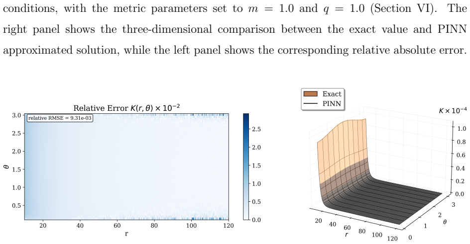
Evaluate the Kretschmann scalar from the relaxed-boundary $q=1$ PINN solution on a dense independent grid in the innermost subdomain $r\in(10m,18m)$, $\theta\in(0,\pi)$, and compare it with the exact q-metric value; if the Einstein residual loss is low but the relative error of this invariant is far above $10^{-3}$ in that region, the claim that the residuals alone select the physical solution is falsified.
Extended reading notes
Core claim
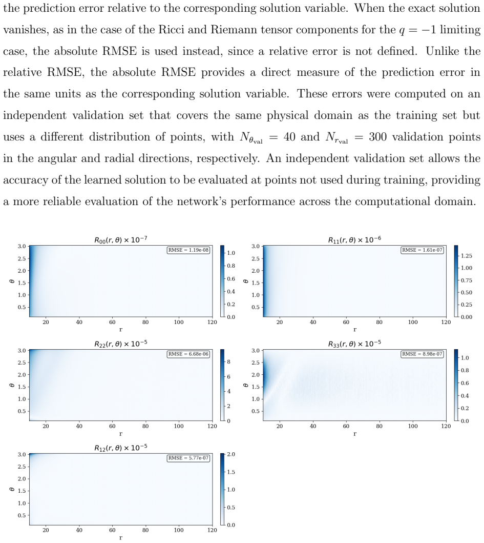
The paper's central claim is that Einstein's vacuum field equations $R_{\mu\nu}=0$ for static spacetimes can be solved directly by physics-informed neural networks, and that the method extends from the spherically symmetric Schwarzschild metric to the axisymmetric q-metric, the simplest exact vacuum solution with a quadrupole moment. In the strict boundary-condition setup, where all four metric functions are pinned to their known asymptotic correction form at the outer boundary, the network reproduces the q-metric with relative RMSE below $10^{-6}$. When those boundary conditions are relaxed so that only the outermost radial subdomain carries boundary data and the inner subdomains are trained from the Einstein residuals alone, the four metric functions are still recovered with relative RMSE between $10^{-6}$ and $10^{-4}$. The paper also shows that in the flat limit $q=-1$, where the network must learn a coordinate representation of Minkowski space rather than the standard line element, the Riemann tensor components reconstructed from the network have $L^\infty$ errors of order $10^{-4}$, which it interprets as residual numerical curvature rather than physical curvature.
Load-bearing premise
The relaxed boundary-condition scheme assumes that a neural network trained on the Einstein residuals alone in the inner radial subdomains, with boundary data supplied only at the outermost edge and passed inward by sequential training, will select the true physical metric rather than another Ricci-flat geometry; the paper itself warns that a low loss value does not guarantee the physical solution.
Editorial extensions
If this is right
- An axisymmetric vacuum spacetime with a quadrupole moment can be recovered from Einstein's equations by a PINN without any mesh, at relative errors competitive with conventional numerical schemes.
- Boundary data need not be supplied throughout the domain: sequential domain decomposition lets the outermost boundary conditions propagate inward while inner subdomains are constrained only by the field equations.
- Validation by invariants such as the Ricci tensor and Kretschmann scalar is necessary, because the same physical spacetime may be represented in different coordinate forms by the network.
- The same architecture and training schedule can be pointed at spacetimes with no known exact solution, using asymptotic or matched-interior boundary data.
- Redundant Einstein equations need not be discarded; their effect can be absorbed through loss weights, simplifying the setup for more complex metrics.
Reading between the lines
- An extension the paper does not test is dropping the angular periodic boundary conditions as well as the inner radial ones; if the relaxed scheme still converges to the q-metric, boundary information enters only through the outermost edge, which would strengthen the method for genuinely unknown domains.
- The residual Riemann curvature measured in the flat-limit case suggests a general acceptance test for PINN solutions in general relativity: compute the $L^\infty$ norm of an invariant curvature scalar and require it to track the exact value, not just the loss.
- The sequential weight-transfer scheme resembles a continuation method; one might initialize the inner subdomains with the outer solution and anneal a source term, which is a different route to stabilizing strong-gradient regions near $r=2m$.
- If the approach extends to time-dependent or non-static spacetimes, the same boundary-relaxation idea could reduce the burden of specifying initial and boundary data in numerical relativity, though that extension is not established here.
Signed reviews
Editorial analysis
A structured set of objections, weighed in public.
Referee Report
Summary. The paper applies physics-informed neural networks (PINNs) to the vacuum Einstein equations for two static spacetimes. For Schwarzschild it reproduces the metric functions using a domain-decomposed PINN and reports RMSE values. For the q-metric it introduces a parametrized ansatz with four correction fields, compares 'strict' and 'relaxed' boundary-condition strategies, and reports that the metric functions are recovered with relative RMSE below 1e-4 for q=1 and below 1e-6 for q=-1, with additional validation via Ricci and Riemann tensor components and the Kretschmann scalar. The paper concludes that PINNs are robust and flexible for solving Einstein's equations and promising for configurations without known analytical solutions.
Significance. If fully supported, the paper would be a useful benchmark showing how boundary conditions and domain decomposition affect PINN training in general relativity. The Schwarzschild test is a genuine forward problem and the numerical setup is documented in enough detail to allow reproduction. The additional validation using curvature invariants is good practice. However, as argued in Major Comment 1, the q-metric experiments embed the exact solution in the ansatz, so they do not test the network's ability to discover unknown spacetimes. The abstract and conclusions therefore overstate the significance for configurations without known analytical solutions.
major comments (3)
- [§V, Eqs. (22)–(25) and §VI] The q-metric ansatz is built from the exact q-metric factors, so the exact solution corresponds identically to u_i=0 for all four correction fields. The paper itself states in §VI that the strict boundary conditions 'imply the trivial solution u_i^NN = 0'. Consequently, the q-metric experiments only test whether the network learns to output near-zero corrections, and the RMSE values in Tables II–IV measure deviation from this zero field rather than the ability of the network to discover or represent the q-metric geometry. In the q=-1 case the effect is even stronger: because the exponents 1+q and -1-q vanish in Eqs. (22) and (23), the metric functions A and B are independent of u0 and u1, respectively. This circular construction prevents the experiments from supporting the abstract's claim that the method is a promising foundation for configurations with no known analytical solution. Please either replace the ansatz with a general static axisymmetric metric ansatz that does not contain the exact solution, or substantially narrow the claims.
- [§VII, Fig. 11] In the relaxed boundary-condition scheme, the inner radial subdomains receive no boundary conditions and no interface continuity conditions between subdomains are described; the only connection is the weight initialization propagated from the outermost subdomain. Since the outer-subdomain loss saturates at 1e-2 and the paper itself warns in §VIII that a low loss does not guarantee the physical solution, the claim that Einstein residuals alone select the correct interior solution is not established. Please either impose and document explicit interface conditions, provide a convergence or uniqueness argument for the relaxed scheme, or clearly limit the claim to the specific sequential-initialization protocol used.
- [§II versus §VII.A] The text around Eq. (3) states that 'the limit q=1 corresponds to the flat Minkowski spacetime', but Section VII.A correctly identifies the flat limit as q=-1, consistent with the multipole moments in Eq. (3), which are proportional to (q+1), and with the vanishing Riemann tensor computed there. The q=1 statement is a factual error; the q=1 cases in Sections VI and VII are genuine quadrupole spacetimes, not flat space. Please correct the inconsistency.
minor comments (4)
- [§IX] The Conclusions state that the Schwarzschild temporal and radial components have RMSE of order 1e-3 and 1e-8, respectively, while Table I and §IV report f ~1e-8 and g ~1e-4; please make the numbers consistent.
- [§VII.A] The paragraph discussing the q=-1 error analysis refers to 'Fig. 18' and 'Table III', but the corresponding figure is Fig. 25 and the table is Table IV.
- [§I] The organization paragraph contains 'Section IV III' before presenting the Schwarzschild case; this should read 'Section IV'.
- [Tables II and III and §VI] The captions of Tables II and III call the quantity 'Global mean squared error (RMSE)' while the text describes it as a relative L2 error; please make the terminology consistent. Also, Eqs. (22)–(25) are described as 'strict boundary conditions', but they are actually a parametrization of the metric functions; please clarify explicitly what values of u_i are imposed on the subdomain boundaries in the strict case.
Circularity Check
q-metric 'predictions' reduce to the ansatz: Eqs. (22)-(25) embed the exact q-metric as u_i=0, strict BCs force that trivial solution, and the relaxed case uses the same pre-embedded target.
-
self definitional
[Sec. VI, Eqs. (22)-(25)]
"A(r, θ)^2 = (1 − 2m/r + u0(r, θ)/r^2)^{1+q}, B(r, θ)^2 = (1 − 2m/r + u1(r, θ)/r^2)^{−1−q} (1 + m^2 sin^2 θ/(r^2−2mr))^{−q(q+2)}, C(r, θ)^2 = (1 − 2m/r + u2(r, θ)/r^2)^{−q} (1 + m^2 sin^2 θ/(r^2−2mr))^{−q(q+2)} r^2, D(r, θ)^2 = (1 − 2m/r + u3(r, θ)/r^2)^{−q} r^2 sin^2 θ."
Each metric function is built from the exact q-metric factors with q,m fixed, and the unknown network fields u_i appear only as additive u_i/r^2 corrections. Setting u_i=0 returns precisely Eq. (2), the known q-metric. Thus the target solution is already contained in the network representation by construction. Minimizing the Einstein residuals drives u_i toward zero, so the reported 'reproduction' of the q-metric measures how well the network learns a pre-embedded function, not whether the PINN derived the spacetime from the field equations.
-
fitted input called prediction
[Sec. VI, discussion after Table II]
"This behavior is consistent with the fact that, in the case considered here, the strict boundary conditions imply the trivial solution u_iNN = 0."
The paper admits that the strict boundary conditions force the network output u_i to be identically zero. But u_i=0 is exactly the q-metric by Ansatz (22)-(25). Therefore the high accuracy reported in Table II (RMSE below 1e-6) is the accuracy of a regression to zero in a parametrization that already contains the known solution. The result is forced by the boundary conditions plus the constructed ansatz, not by an independent solution of Einstein's equations.
1 more flagged steps
-
self definitional
[Sec. VII, description of relaxed boundary conditions and Fig. 11]
"Training process begins in the outermost subdomain, where strict boundary conditions are imposed; subsequently, the inner batches, without any boundary conditions, are incorporated into the training."
The relaxed experiment uses the same ansatz (22)-(25), so the exact q-metric is still u_i=0. Only the outer batch receives boundary data; inner batches are trained on residuals plus weight initialization, with no interface constraints. The RMSE in Table III therefore still measures convergence to a solution that was put into the network by construction. This cannot support the paper's claim of readiness for configurations with no known analytical solution, especially since Sec. VIII warns that a loss of order 1e-2 need not correspond to the physical solution.
full rationale
The circularity is concentrated in the q-metric sections (VI-VII). Equations (22)-(25) define all four metric functions using the known q-metric factors, which makes u_i=0 the exact Einsteinian solution. The paper explicitly acknowledges that strict boundary conditions force this trivial solution, and the relaxed case simply moves the boundary data to the outermost subdomain without changing the pre-embedded target. Consequently, Tables II-IV report how well the network fits a solution that is already present in the ansatz, not evidence that the method discovers unknown spacetimes. The abstract's conclusion that PINNs 'offer a promising foundation for investigating gravitational configurations for which exact analytical solutions are unknown' is an extrapolation beyond what these benchmarks can show, since every q-metric experiment contains the exact answer by construction. The Schwarzschild benchmark is less problematic: the ansatz f=1-2m/r-u0/r^2, g=u1 does not embed the exact g, and the reported RMSE of order 1e-4 for g gives the method some independent validation. The cited q-metric background from Quevedo [7] is standard self-citation but is not the mechanism of circularity here. Overall, the central showcase result reduces by construction to regression toward the known solution, giving a partial but real circularity score of 7 rather than higher because the network could in principle fail to converge and the Schwarzschild test has independent content.
Assumptions & free parameters
assumptions (3)
- domain assumption The q-metric (Eq. 2) is an exact vacuum solution of Einstein's equations with the stated multipole moments.
- standard math For a static spherically symmetric metric, R_theta_theta=0 is redundant given R_tt=0 and R_rr=0, due to Bianchi identities.
- ad hoc to paper The PINN ansatz (22)-(25) is sufficient to represent the target q-metric.
Cite this review
Pith. "Pith review of Solving Einstein's Vacuum Equations with Physics-Informed Neural Networks: Boundary Conditions and Domain Decomposition." pith.science (2026). https://pith.science/paper/CQ7QWINP
@misc{pith2026260808846,
  author       = {Pith},
  title        = {Pith review of: Solving Einstein's Vacuum Equations with Physics-Informed Neural Networks: Boundary Conditions and Domain Decomposition},
  year         = {2026},
  howpublished = {\url{https://pith.science/paper/CQ7QWINP}},
  note         = {Machine review of arXiv:2608.08846}
}
abstract
We investigate the application of Physics-Informed Neural Networks (PINNs) to the numerical solution of Einstein's vacuum field equations for static spacetimes. We first reproduce the Schwarzschild solution and then extend the method to the axisymmetric $q-$metric, a nontrivial exact solution characterized by a mass quadrupole moment. We analyze the influence of boundary conditions, domain decomposition, and equation redundancy on the convergence and stability of the training process. The proposed framework accurately reconstructs the metric functions in the computational domain while maintaining small residual errors. Our results demonstrate that PINNs provide a robust and flexible approach to solving Einstein's equations and offer a promising foundation for investigating gravitational configurations for which exact analytical solutions are unknown.
Figures


Figures from the paper (26 more)




Reference graph
Works this paper leans on
-
[1]
G. E. Karniadakis, I. G. Kevrekidis, L. Lu, P. Perdikaris, S. Wang, and L. Yang, Nature Reviews Physics3, 422 (2021)
2021
- [2]
-
[3]
Raissi, P
M. Raissi, P. Perdikaris, and G. E. Karniadakis, Journal of Computational Physics378, 686 (2019)
2019
- [4]
-
[5]
P. Stefanou, J. F. Urb´ an, and J. A. Pons, Monthly Notices of the Royal Astronomical Society 526, 1504 (2023)
work page 2023
- [6]
-
[7]
The geometric and physical properties of this metric have been in- vestigated in detail in [7, 9–14]
given by ds2 =− 1− 2m r 1+q dt2 + 1− 2m r −q × " 1 + m2 sin2 θ r2 −2mr −q(q+2) r2dθ2 + dr2 1−2m/r +r 2 sin2 θ dφ2 # .(2) The q-metric is obtained from the Schwarzschild metric by applying a Zipoy-Voorhees transformation [8, 9]. The geometric and physical properties of this metric have been in- vestigated in detail in [7, 9–14]. The deformation of the grav...
work page 2000
-
[8]
Quevedo, International Journal of Modern Physics D20, 1779 (2011)
H. Quevedo, International Journal of Modern Physics D20, 1779 (2011)
work page 2011
Show all 20 references
-
[9]
D. M. Zipoy, Journal of Mathematical Physics7, 1137 (1966)
1966
-
[10]
Voorhees, Physical Review D2, 2119 (1970)
B. Voorhees, Physical Review D2, 2119 (1970)
1970
-
[11]
Hern´ andez-Pastora and J
J. Hern´ andez-Pastora and J. Mart ´ ın, General Relativity and Gravitation26, 877 (1994)
1994
-
[12]
Malafarina, Dynamics and Thermodynamics of Blackholes and Naked Singularities p
D. Malafarina, Dynamics and Thermodynamics of Blackholes and Naked Singularities p. 20 (2004)
2004
-
[13]
Quevedo, inNeutron Stars: Physics Properties and Dynamics, edited by N
H. Quevedo, inNeutron Stars: Physics Properties and Dynamics, edited by N. Takibayev and K. Boshkayev (Nova Science Publishers, 2017), Physics Research and Technology, ISBN 978-1-53610-525-4, 1606.09361
2017 arXiv
-
[14]
Frutos-Alfaro, H
F. Frutos-Alfaro, H. Quevedo, and P. A. Sanchez, Royal Society Open Science5, 170826 (2018)
2018
-
[15]
Boshkayev, E
K. Boshkayev, E. Gasperin, A. Guti´ errez-Pi˜ neres, H. Quevedo, and S. Toktarbay, Physical Review D93, 024024 (2016)
2016
-
[16]
Geroch, Journal of Mathematical Physics11, 1955 (1970)
R. Geroch, Journal of Mathematical Physics11, 1955 (1970)
1970
-
[17]
Geroch, Journal of Mathematical Physics11, 2580 (1970)
R. Geroch, Journal of Mathematical Physics11, 2580 (1970). 45
1970
-
[18]
Griewank and A
A. Griewank and A. Walther,Evaluating Derivatives: Principles and Techniques of Algorith- mic Differentiation(SIAM, 2008), 2nd ed
2008
-
[19]
Bradbury, R
J. Bradbury, R. Frostig, P. Hawkins, et al. (2018), http://github.com/google/jax
2018
-
[20]
Alcubierre,Introduction to 3+ 1 numerical relativity, vol
M. Alcubierre,Introduction to 3+ 1 numerical relativity, vol. 140 (OUP Oxford, 2008). 46
2008
Reviewed August 14, 2026 · model on record in the stance chip above.
Discussion (0). Continue with ORCID to comment.