REVIEW 3 major objections 6 minor 79 references
Two-Step MV-DeepONet: Probabilistic Operator Learning for Uncertainty Propagation Driven by Random Input Fields
T0 review · 3 major / 6 minor · reviewed 2026-08-12 · deepseek-v4-flash
Pith's one-line read A two-step probabilistic DeepONet models uncertainty in a low-dimensional coefficient space and recovers cross-location output covariance in a single forward pass, with an error bound tied to four identifiable factors.
desk verdict A genuinely useful extension of Prob-DeepONet: the paper moves Gaussian NLL training into a rotated low-dimensional coefficient space and thereby induces non-diagonal conditional covariance in the output field, but the fixed-basis diagonal-coefficient assumption is a structural prior that the experiments never directly test. read the letter →
The pith
A machine-rendered reading of the paper's core claim, the machinery that carries it, and where it could break.
The reading
What carries the argument
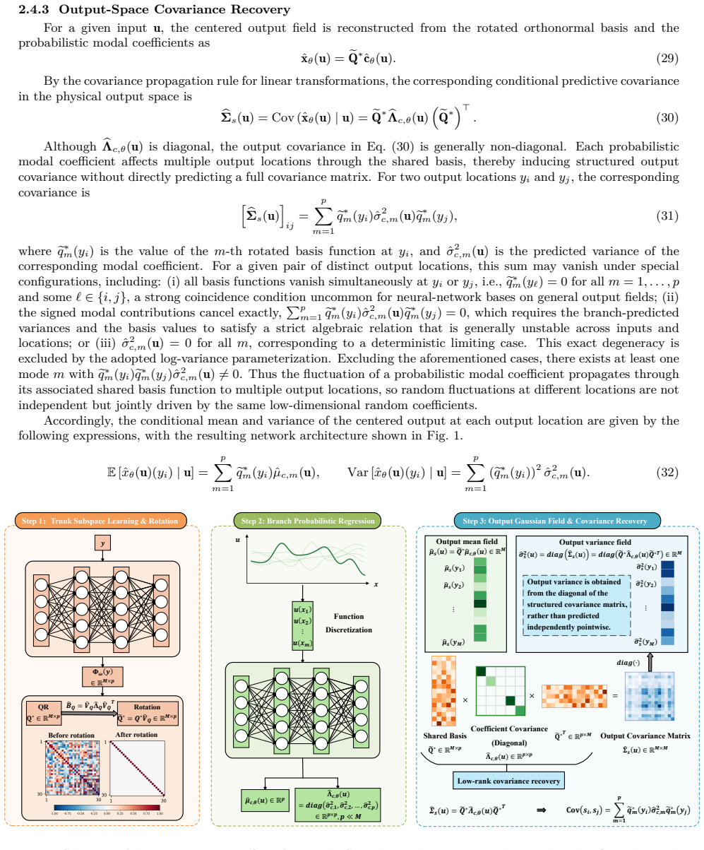
The load-bearing object is the covariance propagation identity $\widehat{\Sigma}_s(u) = \widetilde{Q}^* \widehat{\Lambda}_{c,\theta}(u)(\widetilde{Q}^*)^\top$, which converts a diagonal Gaussian assumption on the rotated modal coefficients into structured output covariance through the shared orthonormal trunk basis $\widetilde{Q}^* \in \mathbb{R}^{M \times p}$ with $p \ll M$. The machinery also includes the two-step training schedule (trunk basis learning first, branch coefficient regression second, with QR orthogonalization and empirical coefficient-covariance diagonalization), and the error analysis built on the Eckart-Young-Mirsky truncation, a spectral-gap bound relating trunk reconstruction risk to subspace distance, and a Davis-Kahan-type finite-sample bound for the empirical eigenspace. Together these components support the claim that covariance recovery is governed by low-rank compressibility, subspace quality, sample size, and branch covariance estimation.
What would settle it
For a fixed test input $u$, draw many solver evaluations (or use a reference surrogate), center the outputs, project them onto the learned rotated basis $\widetilde{Q}^*$, and estimate the conditional coefficient covariance $C = \mathrm{Cov}(c \mid u)$; if the off-diagonal entries of $C$ are not negligible compared with its diagonal entries, then Eq. (30) will miss output correlations and the claimed recovery fails even with a perfect trunk subspace.
Extended reading notes
Core claim
The central claim is that probabilistic modeling in a rotated low-dimensional coefficient space, followed by linear mapping through a shared trunk basis, induces a generally non-diagonal conditional predictive covariance in the physical output space: $\widehat{\Sigma}_s(u) = \widetilde{Q}^* \widehat{\Lambda}_{c,\theta}(u)(\widetilde{Q}^*)^\top$, where $\widehat{\Lambda}_{c,\theta}(u)$ is diagonal. The shared basis is the orthonormal trunk basis after QR orthogonalization and an empirical-covariance eigendecomposition, so each modal coefficient fluctuation reaches multiple output locations and creates cross-location dependence without explicit covariance parameterization. This relaxes the pointwise conditional-independence assumption of Prob-DeepONet while keeping single-pass inference, and the paper argues that the total predictive covariance decomposes by the law of total covariance into a mean-induced part and this structured conditional part. The theoretical analysis further claims that the Frobenius-norm recovery error is bounded by four terms: low-rank truncation of the true output covariance, trunk subspace projection error, finite-sample statistical error, and branch coefficient-covariance estimation error.
Load-bearing premise
The load-bearing premise is that, after the rotation, the modal coefficients are conditionally independent given the input, so the coefficient covariance $\widehat{\Lambda}_{c,\theta}(u)$ can be taken as diagonal; the rotation diagonalizes only the empirical covariance averaged over training samples, not the conditional covariance at each fixed input.
Editorial extensions
If this is right
- A diagonal Gaussian in coefficient space becomes a generally non-diagonal conditional predictive covariance in output space via the shared basis, so cross-location dependence is represented without a full $\mathbb{R}^{M \times M}$ covariance matrix.
- Single-pass inference is retained: the branch network predicts $p$ coefficient means and variances, and the output covariance is obtained by the low-rank product $\widetilde{Q}^* \widehat{\Lambda}_{c,\theta}(u)(\widetilde{Q}^*)^\top$.
- The Frobenius error bound implies that fast spectral decay of the true output covariance, a well-learned trunk subspace separated by a spectral gap, and accurate branch covariance regression are the practical conditions for reliable covariance recovery.
- On the tested reaction-diffusion, Burgers, Darcy, and hypersonic aerothermal problems, the method reports lower out-of-distribution mean errors, more structured uncertainty bands, and accurate multi-anchor correlation maps relative to Prob-DeepONet.
- Conformal calibration brings interval coverage to nominal levels while the two-step model maintains noticeably narrower intervals than the baseline in the reported experiments.
Reading between the lines
- The rotation in the paper diagonalizes the unconditional empirical coefficient covariance over training data; whether the conditional coefficient covariance for a fixed input is also diagonal is a modeling assumption the paper does not prove, and non-diagonal conditional coefficients would change the recovered output correlations.
- A natural extension is to relax the diagonal Gaussian coefficient model to non-Gaussian or correlated latent distributions, since the covariance propagation identity would still map latent dependence into output covariance; the paper lists this direction as future work.
- The framework suggests a general design pattern for operator surrogates: choose any low-dimensional latent distribution, propagate it through a learned linear basis, and obtain an output covariance with structure inherited from the basis, so the method's expressiveness is tied to the quality of the trunk subspace.
- The rank-one aerothermal case illustrates that low-rank covariance is not always easier to recover: with a single dominant mode, Frobenius error is highly sensitive to bias in that mode's variance even when the correlation structure is accurate, so metrics should be read together.
Editorial analysis
A structured set of objections, weighed in public.
Referee Report
Summary. The paper proposes two-step MV-DeepONet, a probabilistic operator-learning model that combines the two-step DeepONet training strategy of Lee and Shin with Gaussian modeling in a low-dimensional rotated coefficient space. The key algebraic device is Eq. (30), where a diagonal input-dependent coefficient covariance is mapped through a learned orthonormal output basis to produce a generally non-diagonal conditional predictive covariance in the physical output space. The authors also provide a Frobenius-norm error decomposition for total predictive covariance recovery, and they validate the method on reaction-diffusion, Burgers, Darcy, and hypersonic aerothermal problems, comparing against Prob-DeepONet in terms of generalization, uncertainty bands, covariance recovery, and calibrated prediction intervals.
Significance. If the central claim holds, the paper offers a lightweight alternative to full covariance parameterization in probabilistic operator learning: it obtains structured conditional covariance while retaining single-pass inference. The construction in Eqs. (22)-(30) is algebraically correct, and the paper is unusually explicit about the decomposition of covariance recovery error into truncation, subspace, statistical, and coefficient-regression terms via Eckart-Young and Davis-Kahan arguments. The empirical study is broad, including three PDE benchmarks and a CFD-based aerothermal problem with a validated solver. The paper also makes a fair comparison setup: covariance recovery is evaluated against held-out empirical covariances, and the branch network minimizes a Gaussian NLL rather than the Frobenius covariance error directly, so the central mechanism is not circular. The main weakness is that the claimed advantage over Prob-DeepONet concerns the conditional predictive covariance, while the numerical evaluation targets the total predictive covariance, for which no ground-truth conditional object exists in the deterministic benchmarks.
major comments (3)
- [Section 2.4.2, Eq. (27)] The diagonal form of the conditional coefficient covariance is an input assumption, not a consequence of the rotation in Eq. (22). The rotation diagonalizes the unconditional empirical coefficient covariance over the training set; for a fixed input u it does not diagonalize the conditional covariance of the coefficient residuals, and the eigenvectors of that conditional covariance may vary with u. The model class in Eq. (30) is therefore restricted to matrices of the form eQ* diag(sigma^2) eQ*^T. If the true conditional coefficient covariance has non-negligible off-diagonal entries, the predicted off-diagonal output correlations are misspecified. Since the misspecification is absorbed into the unquantified term eta_B_app in Eq. (65), the analysis does not control the error caused by the central modeling assumption. A concrete diagnostic would be to estimate the conditional covariance of the coefficient residuals in fixed input bins, or to test on a synthetic problem with known non-diagonal conditional coefficient covariance.
- [Section 3, Eq. (70) and Sections 3.1.2-3.4.2] The numerical evaluation compares the total predictive covariance bSigma_2step of Eq. (37) with the empirical total covariance of the test outputs, not the conditional covariance bSigma_s(u) of Eq. (30). Because the PDE and CFD maps in these benchmarks are deterministic, there is no ground-truth conditional covariance of s(u)|u against which to validate Eq. (30); the non-diagonality of the reference covariance arises from variation of the conditional means across inputs, i.e., the first term in the law of total covariance, Eq. (14). The reported Frobenius errors and correlation maps therefore cannot substantiate the paper's claim that the method recovers off-diagonal conditional dependence. I recommend adding either a benchmark with repeated output realizations for the same input (for example noisy observations or stochastic PDE outputs), or a held-out residual analysis that decomposes the total covariance error into the contributions of bB_mu and bB_sigma, together with a correlation-map comparison against Prob-DeepONet's total covariance.
- [Section 2.4.4, Eqs. (65)-(69)] The presentation calls Eq. (69) an upper bound, but eta_B_app and eta_B_opt are defined as the deviations of the trained model from a best-in-class model and are never estimated or dominated by computable quantities. The recovered error hierarchy T1 << T2, T3 << T2 reported in Sections 3.1.2, 3.2.2, and 3.3.2 is inferred from the gap between the oracle curve and the final model curve; that gap is precisely the unquantified model-dependent error. The theory would be substantially stronger if the approximation term were bounded or estimated, or if the misspecification in Eq. (27) were isolated in a separate term that the experiments explicitly control.
minor comments (6)
- [Eqs. (32) and (41)] The prediction equations describe the centered output only; the paper should state explicitly that the reported mean predictions in Figures 4, 9, 14, and 21 are obtained by adding the training mean from Eq. (19) to eQ* times the predicted coefficient mean.
- [Section 2.4.3, Eq. (31)] The argument that the covariance is nonzero excludes only the case where all basis functions vanish simultaneously at one of the two locations; a complementary pattern in which some modes vanish at y_i and other modes vanish at y_j is still logically possible. A generic-density or non-vanishing-product assumption would make the argument complete.
- [Section 3, ensemble usage] The paper does not report the network widths, depths, learning rates, optimizer settings, or the ensemble aggregation rule for the eight-member ensembles shown in the training-loss figures; because the numerical results appear to depend on these ensembles, the experiments are difficult to reproduce without this information.
- [Figures 2, 3, 7, 8, 12, 13, 18, 19] The axis labels use a pound sign where a multiplication sign is intended; the labels should read 'Epochs (x 10^3)' or similar.
- [Section 3.1.1, Table 2] The 'mean error' over out-of-distribution correlation lengths is an unweighted average over an irregular grid of ell values; the averaging convention should be stated.
- [Section 3.4 and Appendix B] The aerothermal example varies only the freestream Mach number, and Appendix B shows that the effective stochastic dimension is one; the paper should acknowledge that this case is not a test of high-dimensional input-field uncertainty propagation in the same sense as the PDE benchmarks.
Circularity Check
No circularity: the non-diagonal conditional covariance in Eq. (30) follows by exact covariance propagation from a diagonal coefficient-space model; the rotation is a standard training-set representation and is not used as a substitute for the prediction target.
full rationale
The paper's central construction is algebraic rather than circular. Eq. (30), Sigma_s(u) = eQ* Lambda_c,theta(u) (eQ*)^T, is the definition of the output covariance of the linear map x_hat(u) = eQ* c_hat(u); a diagonal Lambda produces a generally non-diagonal output covariance, so the stated result is a consequence of the model specification, not a hidden reuse of the target. The rotation in Eq. (22) diagonalizes the unconditional empirical coefficient covariance over training outputs; this is representation learning (a PCA-type coordinate change), and the paper never claims it makes the conditional coefficient covariance diagonal. The diagonal conditional coefficient covariance in Eq. (27) is an explicitly stated modeling assumption, and Section 4 identifies non-Gaussian conditional structure as future work; an unverified assumption is a limitation of model fidelity, not circularity. The error bound in Eqs. (50)-(69) is a standard triangle-inequality decomposition into truncation, subspace, statistical, and branch terms; it does not assume the quantity being bounded. The two-step training and Theorem 3.5 are cited to Lee and Shin [45], an external reference, and no self-citation is load-bearing. Numerical evaluation compares the model covariance to the held-out test empirical covariance, so the covariance claim is independently checked rather than fitted by construction.
Assumptions & free parameters
free parameters (4)
- Number of retained modes p =
varies per case (e.g., up to 120 for reaction-diffusion, 200 for Burgers)
- VAE latent dimension dz =
64
- KL regularization weight lambda_KL =
1e-4
- Physics-informed weighting strength epsilon =
1.0
assumptions (3)
- domain assumption The true covariance spectral gap gamma_p = lambda_p - lambda_{p+1} is non-vanishing.
- domain assumption Standard covariance concentration conditions give ||Sigma_hat - Sigma||_2 = OP(K^{-1/2}).
- ad hoc to paper The conditional covariance of modal coefficients in the rotated space is diagonal (independence of coefficients given input).
Cite this review
Pith. "Pith review of Two-Step MV-DeepONet: Probabilistic Operator Learning for Uncertainty Propagation Driven by Random Input Fields." pith.science (2026). https://pith.science/paper/B2SHNH2G
@misc{pith2026260809071,
  author       = {Pith},
  title        = {Pith review of: Two-Step MV-DeepONet: Probabilistic Operator Learning for Uncertainty Propagation Driven by Random Input Fields},
  year         = {2026},
  howpublished = {\url{https://pith.science/paper/B2SHNH2G}},
  note         = {Machine review of arXiv:2608.09071}
}
read the original abstract
Forward uncertainty propagation in complex physical systems can induce structured covariance across field-valued outputs. For a probabilistic surrogate, the total predictive covariance comprises the covariance of conditional means across input realizations and the average conditional predictive covariance. Probabilistic DeepONet (Prob-DeepONet) provides lightweight uncertainty quantification by predicting pointwise Gaussian means and variances in a single forward pass, but its conditional predictive covariance is restricted to a diagonal form. To represent cross-location conditional dependence without explicitly parameterizing a full high-dimensional covariance matrix, we develop a two-step mean-variance DeepONet (two-step MV-DeepONet) through two principal modifications. First, two-step training is used to decouple output-basis learning from the input-to-coefficient mapping, together with basis orthogonalization and subspace rotation. Second, Gaussian probabilistic modeling is transferred from the high-dimensional physical output space to the low-dimensional rotated coefficient space. Mapping these probabilistic coefficients through the shared basis induces a generally non-diagonal conditional predictive covariance in the physical output space while retaining single-pass inference. A Frobenius-norm error decomposition and corresponding upper bound identify low-rank covariance compressibility, trunk-subspace approximation, finite-sample statistical error, and coefficient-space covariance estimation as the principal factors governing covariance recovery. Numerical experiments on three representative problems governed by partial differential equations (PDEs) and a hypersonic blunt-body aerothermal problem show improved generalization, more structured uncertainty bands, and accurate recovery of off-diagonal correlation patterns compared with Prob-DeepONet.
Figures


Figures from the paper (22 more)


Reference graph
Works this paper leans on
-
[1]
S. Mohammadi, S. Cremaschi, Efficiency of uncertainty propagation methods for moment estimation of uncertain model outputs, Comput. Chem. Eng. 166 (2022) 107954
work page 2022
-
[2]
W. Liu, T. Belytschko, A. Mani, Random field finite elements, Int. J. Numer. Methods Eng. 23 (1986) 1831–1845
work page 1986
-
[3]
D. Xiu, G. Karniadakis, A new stochastic approach to transient heat conduction modeling with uncertainty, Int. J. Heat Mass Transfer 46 (2003) 4681–4693
work page 2003
-
[4]
I. Simpson, S. Vicente, N. Campbell, Learning structured Gaussians to approximate deep ensembles, in: 2022 IEEE/CVF Conference on Computer Vision and Pattern Recognition (CVPR), IEEE, 2022, pp. 366–374
work page 2022
-
[5]
S. Lee, W. Chen, A comparative study of uncertainty propagation methods for black-box-type problems, Struct. Multidiscip. Optim. 37 (2009) 239–253
work page 2009
-
[6]
K. Abdi, B. Celse, K. McAuley, Propagating input uncertainties into parameter uncertainties and model prediction uncertainties—A review, Can. J. Chem. Eng. 102 (2024) 254–273
work page 2024
- [7]
-
[8]
D. Xiu, G. Karniadakis, The Wiener–Askey polynomial chaos for stochastic differential equations, SIAM J. Sci. Comput. 24 (2002) 619–644
work page 2002
Show all 79 references
-
[9]
D. Xiu, J. Hesthaven, High-order collocation methods for differential equations with random inputs, SIAM J. Sci. Comput. 27 (2005) 1118–1139
2005
-
[10]
Petersen, A
F. Petersen, A. Mishra, H. Kuehne, C. Borgelt, O. Deussen, M. Yurochkin, Uncertainty quantification via stable distribution propagation, in: International Conference on Learning Representations, 2024
2024
-
[11]
Shekhovtsov, B
A. Shekhovtsov, B. Flach, Feed-forward propagation in probabilistic neural networks with categorical and max layers, in: International Conference on Learning Representations, 2018
2018
-
[12]
Betancourt, R
D. Betancourt, R. Muhanna, Interval deep learning for computational mechanics problems under input uncertainty, Probab. Eng. Mech. 70 (2022) 103370
2022
-
[13]
A. Sofi, G. Muscolino, F. Giunta, Propagation of uncertain structural properties described by imprecise Probability Density Functions via response surface method, Probab. Eng. Mech. 60 (2020) 103020. 39
2020
-
[14]
Tripathy, I
R. Tripathy, I. Bilionis, M. Gonzalez, Gaussian processes with built-in dimensionality reduction: Applications to high- dimensional uncertainty propagation, J. Comput. Phys. 321 (2016) 191–223
2016
-
[15]
Giannella, F
V. Giannella, F. Bardozzo, A. Postiglione, R. Tagliaferri, R. Sepe, E. Armentani, Neural networks for fatigue crack propagation predictions in real-time under uncertainty, Comput. Struct. 288 (2023) 107157
2023
-
[16]
Gawlikowski, C
J. Gawlikowski, C. R. N. Tassi, M. Ali, J. Lee, M. Humt, J. Feng, A. Kruspe, R. Triebel, P. Jung, R. Roscher, M. Shahzad, W. Yang, R. Bamler, X. X. Zhu, A survey of uncertainty in deep neural networks, Artif. Intell. Rev. 56 (Suppl 1) (2023) 1513–1589
2023
-
[17]
Neal, Bayesian Learning for Neural Networks, Vol
R. Neal, Bayesian Learning for Neural Networks, Vol. 118 of Lecture Notes in Statistics, Springer, New York, 1996
1996
-
[18]
Y. Gal, Z. Ghahramani, Dropout as a Bayesian approximation: Representing model uncertainty in deep learning, in: Proceedings of the 33rd International Conference on Machine Learning, Vol. 48 of Proceedings of Machine Learning Research, 2016, pp. 1050–1059
2016
-
[19]
Lakshminarayanan, A
B. Lakshminarayanan, A. Pritzel, C. Blundell, Simple and scalable predictive uncertainty estimation using deep ensembles, in: Advances in Neural Information Processing Systems, Vol. 30, 2017, pp. 6402–6413
2017
-
[20]
Sensoy, L
M. Sensoy, L. Kaplan, M. Kandemir, Evidential deep learning to quantify classification uncertainty, in: Advances in Neural Information Processing Systems, Vol. 31, 2018, pp. 3179–3189
2018
-
[21]
D. Nix, A. Weigend, Estimating the mean and variance of the target probability distribution, in: Proceedings of the 1994 IEEE International Conference on Neural Networks (ICNN’94), Vol. 1, IEEE, 1994, pp. 55–60
1994
-
[22]
Seitzer, A
M. Seitzer, A. Tavakoli, D. Antic, G. Martius, On the pitfalls of heteroscedastic uncertainty estimation with probabilistic neural networks, in: International Conference on Learning Representations, 2022
2022
-
[23]
Sluijterman, E
L. Sluijterman, E. Cator, T. Heskes, Optimal training of mean variance estimation neural networks, Neurocomputing 597 (2024) 127929
2024
-
[24]
Subedi, A
U. Subedi, A. Tewari, Operator learning: A statistical perspective, Annu. Rev. Stat. Appl. 13 (2026) 123–148
2026
-
[25]
Kovachki, Z
N. Kovachki, Z. Li, B. Liu, K. Azizzadenesheli, K. Bhattacharya, A. Stuart, A. Anandkumar, Neural operator: Learning maps between function spaces with applications to PDEs, J. Mach. Learn. Res. 24 (89) (2023) 1–97
2023
-
[26]
T. Chen, H. Chen, Universal approximation to nonlinear operators by neural networks with arbitrary activation functions and its application to dynamical systems, IEEE Trans. Neural Netw. 6 (4) (1995) 911–917
1995
-
[27]
L. Lu, P. Jin, G. Pang, Z. Zhang, G. E. Karniadakis, Learning nonlinear operators via DeepONet based on the universal approximation theorem of operators, Nat. Mach. Intell. 3 (2021) 218–229
2021
-
[28]
Goswami, A
S. Goswami, A. Bora, Y. Yu, G. Karniadakis, Physics-informed deep neural operator networks, in: T. Rabczuk, K.-J. Bathe (Eds.), Machine Learning in Modeling and Simulation: Methods and Applications, Springer, Cham, 2023, pp. 219–254
2023
-
[29]
Sahin, C
I. Sahin, C. Moya, A. Mollaali, G. Lin, G. Paniagua, Deep operator learning-based surrogate models with uncertainty quantification for optimizing internal cooling channel rib profiles, Int. J. Heat Mass Transfer 219 (2024) 124813
2024
-
[30]
Goswami, M
S. Goswami, M. Yin, Y. Yu, G. E. Karniadakis, A physics-informed variational DeepONet for predicting crack path in quasi-brittle materials, Comput. Methods Appl. Mech. Eng. 391 (2022) 114587
2022
-
[31]
S. Cai, Z. Wang, L. Lu, T. A. Zaki, G. E. Karniadakis, DeepM&Mnet: Inferring the electroconvection multiphysics fields based on operator approximation by neural networks, J. Comput. Phys. 436 (2021) 110296
2021
-
[32]
Z. Mao, L. Lu, O. Marxen, T. A. Zaki, G. E. Karniadakis, DeepM&Mnet for hypersonics: Predicting the coupled flow and finite-rate chemistry behind a normal shock using neural-network approximation of operators, J. Comput. Phys. 447 (2021) 110698
2021
-
[33]
L. Lu, X. Meng, S. Cai, Z. Mao, S. Goswami, Z. Zhang, G. E. Karniadakis, A comprehensive and fair comparison of two neural operators (with practical extensions) based on F AIR data, Comput. Methods Appl. Mech. Eng. 393 (2022) 114778
2022
-
[34]
G. Lin, C. Moya, Z. Zhang, B-DeepONet: An enhanced Bayesian DeepONet for solving noisy parametric PDEs using accelerated replica exchange SGLD, J. Comput. Phys. 473 (2023) 111713
2023
-
[35]
S. Garg, S. Chakraborty, VB-DeepONet: A Bayesian operator learning framework for uncertainty quantification, Eng. Appl. Artif. Intell. 118 (2023) 105685
2023
-
[36]
S. Lone, S. De, R. Nayek, α-VI DeepONet: A prior-robust variational Bayesian approach for enhancing DeepONets with uncertainty quantification, Comput. Methods Appl. Mech. Eng. 449 (2026) 118552
2026
-
[37]
Y. Yang, G. Kissas, P. Perdikaris, Scalable uncertainty quantification for deep operator networks using randomized priors, Comput. Methods Appl. Mech. Eng. 399 (2022) 115399
2022
-
[38]
C. Moya, A. Mollaali, Z. Zhang, L. Lu, G. Lin, Conformalized-DeepONet: A distribution-free framework for uncertainty quantification in deep operator networks, Physica D 471 (2025) 134418
2025
- [39]
-
[40]
L. Ma, L. Guo, H. Wu, T. Zhou, Deep set based operator learning with uncertainty quantification, J. Comput. Phys. 562 (2026) 115011
2026
- [41]
-
[42]
G. Faza, J. Wauters, F. Cuzzolin, H. Hallez, D. Moens, Direct interval propagation methods using neural-network surrogates for uncertainty quantification in physical systems surrogate model, Knowl.-Based Syst. 341 (2026) 115824
2026
-
[43]
C. Moya, S. Zhang, G. Lin, M. Yue, DeepONet-grid-UQ: A trustworthy deep operator framework for predicting the power grid’s post-fault trajectories, Neurocomputing 535 (2023) 166–182
2023
-
[44]
Winovich, M
N. Winovich, M. Daneker, L. Lu, G. Lin, Active operator learning with predictive uncertainty quantification for partial differential equations, J. Comput. Phys. 555 (2026) 114791
2026
-
[45]
S. Lee, Y. Shin, On the training and generalization of deep operator networks, SIAM J. Sci. Comput. 46 (2024) C273–C296
2024
-
[46]
Kiyani, M
E. Kiyani, M. Manav, N. Kadivar, L. D. Lorenzis, G. Karniadakis, Predicting crack nucleation and propagation in brittle materials using deep operator networks with diverse trunk architectures, Comput. Methods Appl. Mech. Eng. 441 (2025) 117984
2025
-
[47]
Jiang, M
Q. Jiang, M. Salvadori, D. Ota, V. Shankar, K. Shukla, Complex valued deep operator network (DeepONet) [ G] for three dimensional Maxwell’s equations: G ∈ Cm×n, J. Comput. Phys. 562 (2026) 114993
2026
-
[48]
H. Jin, B. Zhang, Q. Cao, E. Zhang, A. Bora, S. Krishnaswamy, G. Karniadakis, H. Espinosa, Characterization and inverse design of stochastic mechanical metamaterials using neural operators, Adv. Mater. 37 (2025) 2420063. 40
2025
-
[49]
S. Park, Y. Shin, J. Choo, Deep operator network for surrogate modeling of poroelasticity with random permeability fields, arXiv preprint arXiv:2509.11966 (2025). doi:10.48550/arXiv.2509.11966
2025 doi
-
[50]
Peyvan, V
A. Peyvan, V. Oommen, A. D. Jagtap, G. E. Karniadakis, RiemannONets: Interpretable neural operators for Riemann problems, Comput. Methods Appl. Mech. Eng. 426 (2024) 116996
2024
- [51]
-
[52]
Eckart, G
C. Eckart, G. Young, The approximation of one matrix by another of lower rank, Psychometrika 1 (1936) 211–218
1936
-
[53]
Y. Yu, T. Wang, R. Samworth, A useful variant of the Davis–Kahan theorem for statisticians, Biometrika 102 (2015) 315–323
2015
-
[54]
Koltchinskii, K
V. Koltchinskii, K. Lounici, Concentration inequalities and moment bounds for sample covariance operators, Bernoulli 23 (1) (2017) 110–133
2017
-
[55]
T. Cai, C. Zhang, H. Zhou, Optimal rates of convergence for covariance matrix estimation, Ann. Stat. 38 (2010) 2118–2144
2010
-
[56]
Khosravi, S
A. Khosravi, S. Nahavandi, D. Creighton, A. F. Atiya, Comprehensive review of neural network-based prediction intervals and new advances, IEEE Trans. Neural Netw. 22 (2011) 1341–1356
2011
-
[57]
Fife, Mathematical Aspects of Reacting and Diffusing Systems, Vol
P. Fife, Mathematical Aspects of Reacting and Diffusing Systems, Vol. 28 of Lecture Notes in Biomathematics, Springer, Berlin, Heidelberg, 1979
1979
-
[58]
Aris, The mathematical theory of diffusion and reaction in permeable catalysts, Vol
R. Aris, The mathematical theory of diffusion and reaction in permeable catalysts, Vol. 1: The theory of the steady state, Clarendon Press, Oxford, 1975
1975
-
[59]
Turing, The chemical basis of morphogenesis, Bull
A. Turing, The chemical basis of morphogenesis, Bull. Math. Biol. 52 (1990) 153–197
1990
-
[60]
Cantrell, C
R. Cantrell, C. Cosner, Spatial ecology via reaction–diffusion equations, John Wiley & Sons, Chichester, 2004
2004
-
[61]
England, J
J. England, J. Cardy, Morphogen gradient from a noisy source, Phys. Rev. Lett. 94 (2005) 078101
2005
-
[62]
M. Vlad, D. Rothman, J. Ross, Random channel kinetics for reaction–diffusion systems, Physica D 239 (2010) 739–745
2010
-
[63]
Whitham, Linear and Nonlinear Waves, Wiley, New York, 1974
G. Whitham, Linear and Nonlinear Waves, Wiley, New York, 1974
1974
-
[64]
J. Bec, K. Khanin, Burgers turbulence, Phys. Rep. 447 (2007) 1–66
2007
-
[65]
Buendía, G
G. Buendía, G. Viswanathan, V. Kenkre, Multifractality of random walks in the theory of vehicular traffic, Phys. Rev. E 78 (2008) 056110
2008
-
[66]
Rubin, Applied Stochastic Hydrogeology, Oxford University Press, New York, 2003
Y. Rubin, Applied Stochastic Hydrogeology, Oxford University Press, New York, 2003
2003
-
[67]
Godoy, L
V. Godoy, L. Zuquette, J. Gómez-Hernández, Stochastic analysis of three-dimensional hydraulic conductivity upscaling in a heterogeneous tropical soil, Comput. Geotech. 100 (2018) 174–187
2018
-
[68]
Passiatore, L
D. Passiatore, L. Sciacovelli, P. Cinnella, G. Pascazio, Thermochemical non-equilibrium effects in turbulent hypersonic boundary layers, J. Fluid Mech. 941 (2022) A21
2022
-
[69]
Williams, M
C. Williams, M. D. Renzo, P. Moin, Turbulence–chemistry interaction in a non-equilibrium hypersonic boundary layer, J. Fluid Mech. 1017 (2025) A30
2025
-
[70]
MacLean, E
M. MacLean, E. Marineau, R. Parker, A. Dufrene, M. Holden, P. DesJardin, Effect of surface catalysis on measured heat transfer in expansion tunnel facility, J. Spacecr. Rockets 50 (2013) 470–475
2013
-
[71]
J. B. Dsouza, N. Castelino, V. Viti, H. H. Vu, S. Gao, Numerical study of the effects of thermo-chemical non-equilibrium and surface catalysis on two hypersonic re-entry bodies, in: AIAA SciTech 2024 Forum, AIAA, 2024, AIAA Paper 2024-2086
2024
-
[72]
Park, Assessment of two-temperature kinetic model for ionizing air, J
C. Park, Assessment of two-temperature kinetic model for ionizing air, J. Thermophys. Heat Transf. 3 (1989) 233–244
1989
-
[73]
Gupta, J
R. Gupta, J. Yos, R. Thompson, K.-P. Lee, A review of reaction rates and thermodynamic and transport properties for an 11-species air model for chemical and thermal nonequilibrium calculations to 30000 K, NASA Reference Publication 1232, NASA Langley Research Center, Hampton, ...
1990
-
[74]
Gnoffo, R
P. Gnoffo, R. Gupta, J. Shinn, Conservation equations and physical models for hypersonic air flows in thermal and chemical nonequilibrium, NASA Technical Paper 2867, NASA Langley Research Center, Hampton, V A (1989)
1989
-
[75]
J. A. Rataczak, I. D. Boyd, J. W. McMahon, Surrogate models for hypersonic aerothermodynamics and aerodynamics using gaussian process regression, in: AIAA SciTech 2024 Forum, AIAA, 2024, AIAA Paper 2024-0461
2024
-
[76]
Capriati, A
M. Capriati, A. Cortesi, T. Magin, P. Congedo, Stagnation point heat flux characterization under numerical error and boundary conditions uncertainty, Eur. J. Mech. B Fluids 95 (2022) 221–230
2022
-
[77]
J. Lu, J. Li, Z. Song, W. Zhang, C. Yan, Uncertainty and sensitivity analysis of heat transfer in hypersonic three-dimensional shock waves/turbulent boundary layer interaction flows, Aerosp. Sci. Technol. 123 (2022) 107447
2022
-
[78]
Wright, D
M. Wright, D. Bose, G. Candler, A data parallel line relaxation method for the Navier–Stokes equations, AIAA J. 36 (1998) 1603–1609
1998
-
[79]
P. Jin, S. Meng, L. Lu, MIONet: Learning multiple-input operators via tensor product, SIAM J. Sci. Comput. 44 (6) (2022) A3490–A3514. 41
2022
Reviewed August 12, 2026 · model on record in the stance chip above.
Discussion (0). Continue with ORCID to comment.