REVIEW 2 major objections 4 minor 63 references
Tabular foundation models for the estimation of probabilistic quasar photometric redshifts in S-PLUS
T0 review · 2 major / 4 minor · reviewed 2026-08-14 · deepseek-v4-flash
Pith's one-line read A frozen tabular foundation model, TabPFN 2.5, is the strongest overall probabilistic quasar redshift estimator in S-PLUS DR6.
desk verdict Solid, carefully run benchmark showing TabPFN 2.5 is the best default for S-PLUS quasar photo-z, with the caveat that the covariate-shift calibration claim rests on assumptions the data cannot test. read the letter →
The pith
A machine-rendered reading of the paper's core claim, the machinery that carries it, and where it could break.
The reading
What carries the argument
The load-bearing object is TabPFN 2.5 used as a tabular in-context foundation model: a transformer pre-trained on a large corpus of synthetic tabular regression tasks, applied with frozen weights by supplying the labelled spectroscopic sample as in-context support and reading out a piecewise-constant "bar" distribution over redshift, which is interpolated onto a 200-point redshift grid and renormalised to give a conditional density estimate. The companion machinery is the covariate-shift evaluation: importance weights equal to the ratio of target to source feature densities, estimated by a classifier distinguishing spectroscopic from photometric quasar candidates, tempered with an exponent to control effective sample size, so that weighted metrics approximate performance on the photometric target population. These two pieces together let the paper separate how well a method fits the spectroscopic sample from how well it will behave when deployed on the photometric catalogue.
What would settle it
Obtain spectroscopic redshifts for a random, feature-unselected subsample of the photometric quasar-candidate catalogue and compare the conditional redshift distributions at fixed features with those of the spectroscopic training sample; if they differ measurably, or if removing spectroscopically confirmed non-quasars from the candidate catalogue changes the importance-weighted ranking, the paper's calibration claim for TabPFN 2.5 would be refuted.
Extended reading notes
Core claim
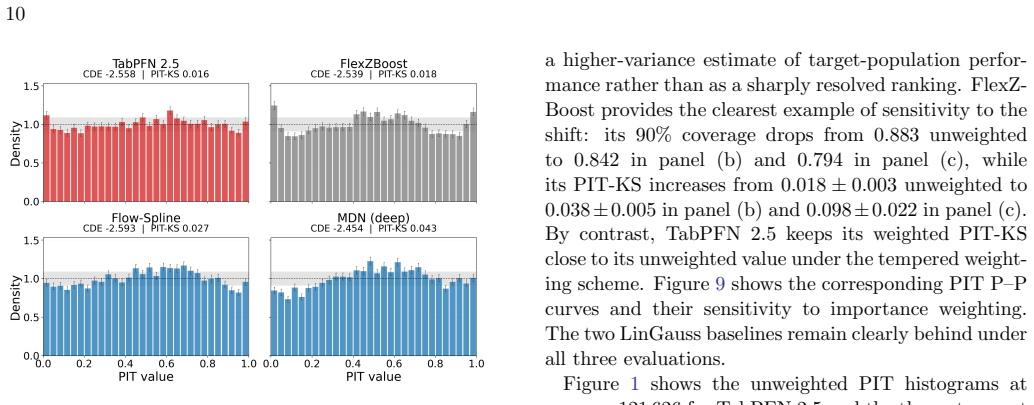
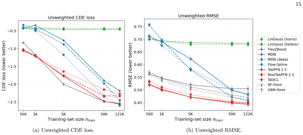
On the paper's own terms, the central discovery is that a transformer pre-trained on synthetic tabular tasks and applied with frozen weights can estimate the conditional redshift density for quasars at least as well as the best task-specific conditional-density estimators, and better in the regimes that matter most. In the benchmark with 121,626 training quasars and 13,538 test quasars, TabPFN 2.5 is best or statistically tied for best on CDE loss, log-likelihood, CRPS, PIT-KS, 90% coverage, RMSE, NMAD, and the catastrophic-outlier fractions; the one exception is unweighted CDE loss, where the normalising flow Flow-Spline is statistically tied and attains the lower mean. Under importance-weighted evaluation toward the photometric candidate population, TabPFN 2.5 remains best or tied for best on essentially all metrics while competitors such as FlexZBoost show degraded coverage, and its PIT-KS stays close to its unweighted value. Its largest gains appear when training sets are small (at most 1,000 objects) and in the low- and high-redshift tails, where catastrophic photo-z failures are most common.
Load-bearing premise
The load-bearing premise is that, at fixed observed photometric features, the redshift distribution of quasars is the same in the spectroscopic sample and the photometric candidate catalogue, and that the candidate catalogue is a sufficiently pure draw from the deployment population; if targeting carries extra information beyond the 39 features, or the catalogue contains non-quasar contaminants, the importance-weighted performance claims are biased.
Editorial extensions
If this is right
- TabPFN 2.5 can serve as a strong default probabilistic photo-z estimator for S-PLUS-like quasar samples, especially when training data are limited or calibrated conditional densities matter.
- The three foundation models are the only methods that stay competitive on catastrophic-outlier fractions under importance-weighted evaluation, so survey pipelines that prioritise outlier control should consider them.
- Method rankings change under covariate-shift weighting: unweighted spectroscopic metrics overstate deployed performance for some baselines, for example FlexZBoost's 90% coverage drops from 0.883 unweighted to 0.794 under raw importance weights.
- Foundation models lead at training sizes of 1,000 or fewer on nearly all metrics; at the full DR6 training size the gap narrows, but TabPFN 2.5 remains among the leading methods.
- SHAP attributions identify WISE W1 and W2 as the strongest individual predictors in TabPFN 2.5, with UV and optical bands providing smaller collective refinements.
Reading between the lines
- If the covariate-shift assumption holds generally, the same frozen-model protocol could transfer to other narrow-band surveys and to galaxies, where multimodality and sample shift are also present; the paper explicitly leaves this extension untested.
- Because TabPFN 2.5's advantage concentrates in sparsely sampled tails, an untested but plausible prediction is that it will also dominate in deeper surveys where the photometric population extends beyond the spectroscopic support.
- The main deployment bottleneck is inference memory, so a practical route would be to distill the frozen model's conditional densities into a cheaper survey-specific emulator; the paper notes distillation as a possible acceleration but does not test it.
- A purity-aware weighting that uses calibrated candidate probabilities instead of a raw candidate catalogue could strengthen or weaken the reported calibration gains; the paper suggests this as future work.
Editorial analysis
A structured set of objections, weighed in public.
Referee Report
Summary. The paper presents a benchmark of three tabular foundation models (TabPFN 2.5, RealTabPFN 2.5, and TabICL) against eight task-specific baselines for probabilistic quasar photometric redshift estimation in S-PLUS DR6. The feature set has 39 dimensions (S-PLUS PSF magnitudes, colours, magnitude errors, WISE W1/W2, and GALEX FUV/NUV); training sizes range from 500 to 121,626 with five repetitions and a fixed test set of 13,538 objects. The evaluation covers density quality (CDE loss, log-likelihood, CRPS, PIT-KS, 90% coverage) and point predictions (RMSE, bias, NMAD, outlier fractions), in both an unweighted mode and an importance-weighted mode designed to approximate the photometric target population, with tempered weights and a sensitivity analysis for the weight estimator. The main finding is that TabPFN 2.5 is best or statistically tied for best on nearly all metrics, with the largest advantages at small training sizes and in difficult regimes; Flow-Spline ties it on unweighted CDE loss. The paper concludes that TabPFN 2.5 is a strong default for S-PLUS-like probabilistic quasar photo-z inference.
Significance. The unweighted benchmark is careful and reproducible: a fixed train/test split inherited from the S-PLUS pipeline, five independent repetitions, per-repetition averaging with test-set bootstrap standard errors, a documented one-SE bold rule, a grid-resolution sensitivity check, and a full re-estimation of importance weights with a different classifier in Appendix C. The result that a frozen in-context foundation model is at least competitive with tuned task-specific density estimators for quasar photo-z is of practical value, especially for small spectroscopic samples, and the paper gives proper credit to the earlier S-PLUS QuCatS pipeline. The fundamental conclusion that TabPFN 2.5 is a strong default in the unweighted, distribution-matched sense is well supported. The deployment-oriented weighted claims, however, inherit the covariate-shift and target-purity assumptions discussed below. This is a benchmark rather than a derivation, and I see no circularity in the reported comparisons.
major comments (2)
- [§3.2 (Eq. 1) and §2.6 (Table 4)] The weighted metrics and the abstract's claim of 'near-nominal calibration under covariate shift' rest on the assumptions that p_s(z|x)=p_t(z|x) and that the DR6 photometric quasar-candidate catalogue is a representative, sufficiently pure draw from the deployment population. Table 4 shows that the target sample is dramatically different from the spectroscopic sample: r is missing for 55.2% of targets, u-r for 94.1%, and W1-W2 for 92.8%, with two-sample KS distances of 0.388-0.655 for the valid measurements. The density-ratio classifier in §3.2.1 therefore separates the samples largely on missingness patterns. If the candidate catalogue contains appreciable non-QSO contamination, or if spectroscopic targeting uses information beyond the 39 features (variability, morphology, ancillary detections), then beta(x) reweights toward a population for which Eq. (1) is undefined or false, and the weighted calibration and outlier-rate conclusions are biased in an unknown direction. Section 5 acknowledges this, but the conclusion still states the weighted behaviour as a property of TabPFN 2.5. Please add a purity-aware analysis (for example, using calibrated candidate probabilities P(QSO|x) as target weights, or sweeping assumed contamination fractions) or explicitly downgrade the weighted claims to conditional-on-purity statements.
- [§3.2.2 (Eq. 5) and Table 2, panel (b)] The headline importance-weighted evaluation uses alpha* ≈ 0.36, chosen to force the effective sample size to 30% of the test set; this is not the target distribution p_t but a variance-reduced interpolation between the spectroscopic and photometric distributions. The alpha = 1 panel, which actually estimates performance on p_t, has ESS ≈ 216 objects (1.6%) and gives TabPFN 2.5 a weighted PIT-KS of 0.064 ± 0.023 and 90% coverage of 0.910 ± 0.015. These numbers do not by themselves establish near-nominal calibration on the target population with meaningful precision. The abstract and Section 5 should be reworded so that 'near-nominal calibration under covariate shift' refers to the tempered interpolation, with target-population calibration reported as a high-variance, assumption-dependent estimate.
minor comments (4)
- [Abstract and Appendix B] The phrase 'statistically tied' corresponds to the one-combined-SE bold rule defined in Appendix B; please add a footnote clarifying that this is a descriptive rule and not a formal equivalence test.
- [Appendix B] The reported standard errors are finite-test-set bootstrap errors after averaging per-object values across the five repetitions; they do not include uncertainty from training-set subsampling. This should be stated explicitly so that readers do not interpret the SEs as full procedure uncertainty.
- [Section 4.4] The SHAP analysis explains only 100 test objects with 83 coalitions per object; the global feature-importance ranking is therefore a rough diagnostic. Please state the sensitivity of the ranking to the number of explained objects and to the coalition budget.
- [Table 4] Because missingness itself is a strong discriminator (94.1% for u-r and 92.8% for W1-W2), the text should note explicitly that the importance-weighted evaluation is reweighting toward objects with incomplete photometry, not only toward fainter or redder objects.
Circularity Check
No significant circularity: the benchmark is a held-out evaluation against fixed spectroscopic redshifts, and the importance weighting is an explicit identity under a stated, untestable covariate-shift assumption rather than a constructed prediction.
full rationale
This paper is a controlled benchmark, not a derivation: TabPFN 2.5, RealTabPFN 2.5, and TabICL are evaluated with frozen weights on a fixed spectroscopic test set with true redshifts, and no metric is produced by fitting the model to the quantity it is claimed to predict. The importance-weighting chain in Section 3.2 is an identity: Eq. (2) follows from the covariate-shift assumption in Eq. (1), and Eq. (4) is the Bayes-rule estimator of beta(x); the weights depend only on the features x and the S=0/S=1 label, not on redshifts or on the photo-z models being ranked. The tempering exponent alpha in Eq. (5) is transparently an evaluation choice, and Appendix C shows that replacing the TabICL weight estimator with gradient boosting leaves the rankings essentially unchanged. Self-citations to Nakazono et al. (2024) for the train/test split and to Izbicki and Lee for FlexZBoost and the CDE loss are methodological anchors rather than load-bearing premises. The paper also flags its real limitation explicitly in Section 5: 'uncertainty in the weights and impurity of the photometric candidate catalogue remain' and 'the covariate-shift assumption may also fail'; Appendix A, Table 4, quantifies the large missingness differences between the spectroscopic and photometric samples. That limitation means the deployment-oriented weighted claim is conditional on an untestable assumption, but it is an external-validity caveat, not a circular reduction of the result to its inputs. No fitted parameter is renamed as a prediction, no uniqueness theorem is imported from the authors' prior work, and no ansatz is smuggled in via self-citation.
Assumptions & free parameters
free parameters (3)
- Tempering exponent alpha =
alpha ≈ 0.36 (ESS target 30%)
- Importance-weight clipping bounds =
[0.01, 0.99]
- Density grid resolution =
200 redshift values (10% expansion)
assumptions (4)
- domain assumption Covariate-shift assumption: p(z|x) is identical in the spectroscopic and photometric target populations (Eq. 1).
- domain assumption Spectroscopic redshifts are exact ground truth with no reported uncertainty and the 1-arcsec cross-match correctly associates counterparts.
- standard math Bayesian and probabilistic identities for density-ratio estimation and proper scoring rules are valid.
- domain assumption TabPFN's pretrained prior provides a valid inductive bias for tabular regression.
Cite this review
Pith. "Pith review of Tabular foundation models for the estimation of probabilistic quasar photometric redshifts in S-PLUS." pith.science (2026). https://pith.science/paper/ITOF5RV5
@misc{pith2026260810280,
  author       = {Pith},
  title        = {Pith review of: Tabular foundation models for the estimation of probabilistic quasar photometric redshifts in S-PLUS},
  year         = {2026},
  howpublished = {\url{https://pith.science/paper/ITOF5RV5}},
  note         = {Machine review of arXiv:2608.10280}
}
read the original abstract
We assess whether tabular foundation models can be used as off-the-shelf probabilistic photometric-redshift estimators for quasars in the 12-band S-PLUS DR6 survey, where colour-redshift degeneracies produce multi-modal posteriors and spectroscopic training sets are shifted relative to the photometric population. TabPFN 2.5, RealTabPFN 2.5, and TabICL are benchmarked against eight task-specific baselines, including linear conditional Gaussians, FlexZBoost, mixture-density networks, normalising flows, random forests, and gradient-boosted trees, with training sets from 500 to 121,626 quasars, using both density and point-prediction metrics, together with importance-weighted scores that approximate deployment on the photometric target sample. TabPFN 2.5 is best or statistically tied for best on all metrics except the unweighted CDE loss, on which the normalising flow is statistically tied and attains the lowest mean value; its largest gains occur for small training sets and in difficult regimes (very bright and faint sources, high redshift), while retaining near-nominal calibration under covariate shift. Its main practical cost is inference: with frozen weights, large support and target catalogues require substantial GPU/accelerator memory, and full-catalogue deployment may need support-set subsampling or distillation. SHAP attributions identify WISE W1/W2 as the strongest individual predictors, with UV and optical bands offering non-negligible refinements. We conclude that TabPFN 2.5 is a strong default for probabilistic quasar photo-z estimation, particularly when training data are limited or when calibration under covariate shift is critical.
Figures


Figures from the paper (7 more)



Reference graph
Works this paper leans on
-
[1]
Abdul Karim, M., Adame, A. G., Aguado, D., et al. 2026, Astronomical Journal, 171, doi: 10.3847/1538-3881/ae4c43
-
[2]
2016, Monthly Notices of the Royal Astronomical Society, 459, 1293
Asorey, J., Carrasco Kind, M., Sevilla-Noarbe, I., Brunner, R., & Thaler, J. 2016, Monthly Notices of the Royal Astronomical Society, 459, 1293
work page 2016
-
[3]
Assef, R. J., Stern, D., Kochanek, C. S., et al. 2013, ApJ, 772, 26, doi: 10.1088/0004-637X/772/1/26
-
[4]
Ball, N., Brunner, R. J., Myers, A., et al. 2008, The Astrophysical Journal, 683, 12, doi: 10.1086/589646
doi:10.1086/589646 2008
-
[5]
2010, in Proceedings of Machine Learning Research, Vol
Ben-David, S., Lu, T., Luu, T., & P´ al, D. 2010, in Proceedings of Machine Learning Research, Vol. 9, Proceedings of the Thirteenth International Conference on Artificial Intelligence and Statistics, 129–136. https://proceedings.mlr.press/v9/david10a.html Ben’ıtez, N., Dupke, R., Moles, M., & et al. 2014, arXiv e-prints
work page 2010
-
[6]
2017, ApJS, 230, 24, doi: 10.3847/1538-4365/aa7053
Bianchi, L., et al. 2017, ApJS, 230, 24, doi: 10.3847/1538-4365/aa7053
-
[7]
2009, Journal of Machine Learning Research, 10, 2137, doi: 10.5555/1577069.1755858
Bickel, S., Br¨ uckner, M., & Scheffer, T. 2009, Journal of Machine Learning Research, 10, 2137, doi: 10.5555/1577069.1755858
arXiv 2009
-
[8]
Bordoloi, R., Lilly, S. J., & Amara, A. 2010, Monthly Notices of the Royal Astronomical Society, 406, 881
work page 2010
Show all 63 references
-
[9]
B., van Dokkum, P
Brammer, G. B., van Dokkum, P. G., & Coppi, P. 2008, The Astrophysical Journal, 686, 1503, doi: 10.1086/591786
2008 doi
-
[10]
2001, Machine Learning, 45, 5, doi: 10.1023/A:1010933404324
Breiman, L. 2001, Machine Learning, 45, 5, doi: 10.1023/A:1010933404324
2001 doi
-
[11]
2013, The Astrophysical Journal, 772, 140, doi: 10.1088/0004-637X/772/2/140
Mercurio, A. 2013, The Astrophysical Journal, 772, 140, doi: 10.1088/0004-637X/772/2/140
2013 doi
-
[12]
J., Mol´ es, M., Crist’obal-Hornillos, D., et al
Cenarro, A. J., Mol´ es, M., Crist’obal-Hornillos, D., et al. 2019, Astronomy & Astrophysics, 622, A176, doi: 10.1051/0004-6361/201833036
2019 doi
-
[13]
2016, in Knowledge Discovery and Data Mining, 785–794, doi: 10.1145/2939672.2939785
Chen, T., & Guestrin, C. 2016, in Knowledge Discovery and Data Mining, 785–794, doi: 10.1145/2939672.2939785
2016
-
[14]
E., Lima, M., Oyaizu, H., Frieman, J., & Lin, H
Cunha, C. E., Lima, M., Oyaizu, H., Frieman, J., & Lin, H. 2009, Monthly Notices of the Royal Astronomical Society, 396, 2379
2009
-
[15]
B., et al
Dalmasso, N., Pospisil, T., Lee, A. B., et al. 2020, Astronomy and Computing, 30, 100362 27 DESI Collaboration, Aghamousa, A., Aguilar, J., et al. 2016, arXiv e-prints
2020
-
[16]
H., et al
Dey, B., Zhao, D., Andrews, B. H., et al. 2025, Machine Learning: Science and Technology, 6, 045058
2025
-
[17]
A., Bovy, J., Myers, A
DiPompeo, M. A., Bovy, J., Myers, A. D., & Lang, D. 2015, Monthly Notices of the Royal Astronomical Society, 452, 3124–3138, doi: 10.1093/mnras/stv1562
2015 doi
-
[18]
2019, in Neural Information Processing Systems
Durkan, C., Bekasov, A., Murray, I., & Papamakarios, G. 2019, in Neural Information Processing Systems. https://arxiv.org/abs/1906.04032
2019 arXiv
-
[19]
2023, Annual Review of Astronomy and Astrophysics, 61, 373, doi: 10.1146/annurev-astro-052920-102455
Fan, X., Ba˜ nados, E., & Simcoe, R. 2023, Annual Review of Astronomy and Astrophysics, 61, 373, doi: 10.1146/annurev-astro-052920-102455
2023 doi
-
[20]
Freeman, P., Izbicki, R., & Lee, A. B. 2017, Monthly notices of the Royal Astronomical Society, 468, 4556, doi: 10.1093/mnras/stx764
2017 doi
- [21]
-
[22]
2007, Journal of the American Statistical Association, 102, 359, doi: 10.1198/016214506000001437
Gneiting, T., & Raftery, A. 2007, Journal of the American Statistical Association, 102, 359, doi: 10.1198/016214506000001437
2007 doi
- [23]
-
[24]
2022, in Proceedings of Machine Learning Research, Vol
Gulrajani, I., & Hashimoto, T. 2022, in Proceedings of Machine Learning Research, Vol. 162, Proceedings of the 39th International Conference on Machine Learning, 7982–7997. https://proceedings.mlr.press/v162/gulrajani22a.html
2022
-
[25]
2014, Annual Review of Astronomy and Astrophysics, 52, 589, doi: 10.1146/annurev-astro-081913-035722
Heckman, T., & Best, P. 2014, Annual Review of Astronomy and Astrophysics, 52, 589, doi: 10.1146/annurev-astro-081913-035722
2014 doi
-
[26]
Herpich, F., Almeida-Fernandes, F., Schwarz, G. B. O., et al. 2024, Astronomy & Astrophysics, 689, A249, doi: 10.1051/0004-6361/202449725
2024 doi
-
[27]
2017, The Astrophysical Journal, 849, 53, doi: 10.3847/1538-4357/aa8c77
Hickox, R., Myers, A., Greene, J., et al. 2017, The Astrophysical Journal, 849, 53, doi: 10.3847/1538-4357/aa8c77
2017 doi
-
[28]
2010, Astronomy & Astrophysics, 523, A31, doi: 10.1051/0004-6361/201014885
Hildebrandt, H., Arnouts, S., Capak, P., et al. 2010, Astronomy & Astrophysics, 523, A31, doi: 10.1051/0004-6361/201014885
2010 doi
-
[29]
G., Purucker, L., et al
Hollmann, N., M¨ uller, S. G., Purucker, L., et al. 2025, Nature, 637, 319, doi: 10.1038/s41586-024-08328-6
2025 doi
-
[30]
2025, Machine Learning Beyond Point Predictions: Uncertainty Quantification, 1st edn., 260
Izbicki, R. 2025, Machine Learning Beyond Point Predictions: Uncertainty Quantification, 1st edn., 260
2025
-
[31]
2014, in Artificial intelligence and statistics, PMLR, 420–429
Izbicki, R., Lee, A., & Schafer, C. 2014, in Artificial intelligence and statistics, PMLR, 420–429
2014
-
[32]
Izbicki, R., & Lee, A. B. 2016, Journal of Computational and Graphical Statistics, 25, 1297
2016
-
[33]
Izbicki, R., & Lee, A. B. 2017, Electronic Journal of Statistics, 11, 2800, doi: 10.1214/17-EJS1302
2017 doi
-
[34]
B., & Freeman, P
Izbicki, R., Lee, A. B., & Freeman, P. 2017, Annals of Applied Statistics, 11, 698, doi: 10.1214/16-AOAS1013
2017 doi
-
[35]
Izbicki, R., & Rodrigues, P. L. C. 2026, arXiv e-prints, arXiv:2603.26611, doi: 10.48550/arXiv.2603.26611
2026 doi
- [36]
-
[37]
2025, ErikVini/specz compilation: Southern Hemisphere Spectrocopic Redshift Compilation, 2025.03.27 Zenodo, doi: 10.5281/zenodo.15127060
Lima, E. 2025, ErikVini/specz compilation: Southern Hemisphere Spectrocopic Redshift Compilation, 2025.03.27 Zenodo, doi: 10.5281/zenodo.15127060
2025 doi
-
[38]
2001, ARA&A, 39, doi: 10.1146/annurev.astro.39.1.19
Loeb, A., & Barkana, R. 2001, ARA&A, 39, doi: 10.1146/annurev.astro.39.1.19
2001 doi
-
[39]
M., & Lee, S.-I
Lundberg, S. M., & Lee, S.-I. 2017, in Neural Information Processing Systems, Vol. 30
2017
-
[40]
2008, MNRAS, 386, 781, doi: 10.1111/j.1365-2966.2008.12947.x
Mandelbaum, R., Seljak, U., Hirata, C., et al. 2008, MNRAS, 386, 781, doi: 10.1111/j.1365-2966.2008.12947.x
2008
-
[41]
C., et al
Martin, D. C., et al. 2005, ApJL, 619, L1, doi: 10.1086/426387 Mendes de Oliveira, C., Ribeiro, T., Schoenell, W., et al. 2019, Monthly Notices of the Royal Astronomical Society, 489, 241, doi: 10.1093/mnras/stz1985
2005 doi
-
[42]
2007, ApJS, 173, 682, doi: 10.1086/520512
Morrissey, P., et al. 2007, ApJS, 173, 682, doi: 10.1086/520512
2007 doi
-
[43]
2016, in Astrophysics and Space Science
Mortlock, D. 2016, in Astrophysics and Space Science
2016
-
[44]
423, Understanding the Epoch of Cosmic Reionization: Challenges and Progress, ed
Library, Vol. 423, Understanding the Epoch of Cosmic Reionization: Challenges and Progress, ed. A. Mesinger, 187–226, doi: 10.1007/978-3-319-21957-8 7
- [45]
-
[46]
2009, Monthly Notices of the Royal Astronomical Society, 399, 2279, doi: 10.1111/j.1365-2966.2009.15432.x
Myers, A., White, M., & Ball, N. 2009, Monthly Notices of the Royal Astronomical Society, 399, 2279, doi: 10.1111/j.1365-2966.2009.15432.x
2009
-
[47]
Nakazono, L., Oliveira, C. M. d., Hirata, N., et al. 2021, Monthly notices of the Royal Astronomical Society, 507, 5847, doi: 10.1093/mnras/stab1835
2021 doi
-
[48]
R., Soares, G., et al
Nakazono, L., Valencca, R. R., Soares, G., et al. 2024, Monthly notices of the Royal Astronomical Society, 531, 327, doi: 10.1093/mnras/stae971
2024 doi
-
[49]
2016, arXiv e-prints
Polsterer, K., D’Isanto, A., & Gieseke, F. 2016, arXiv e-prints
2016
- [50]
-
[51]
2023, Monthly notices of the Royal Astronomical Society, 524, doi: 10.1093/mnras/stad1962
Rau, M., Dalal, R., Zhang, T., et al. 2023, Monthly notices of the Royal Astronomical Society, 524, doi: 10.1093/mnras/stad1962
2023 doi
-
[52]
T., Fan, X., Schneider, D
Richards, G. T., Fan, X., Schneider, D. P., et al. 2001, The Astronomical Journal, 121, 2308 28
2001
-
[53]
2024, in World Conference on Explainable Artificial Intelligence, Springer, 465–476
Rundel, D., Kobialka, J., von Crailsheim, C., et al. 2024, in World Conference on Explainable Artificial Intelligence, Springer, 465–476
2024
-
[54]
2019, Nature Astronomy, 3, 212, doi: 10.1038/s41550-018-0478-0
Salvato, M., Ilbert, O., & Hoyle, B. 2019, Nature Astronomy, 3, 212, doi: 10.1038/s41550-018-0478-0
2019 doi
- [55]
-
[56]
2020, Monthly notices of the Royal Astronomical Society, 499, 1587, doi: 10.1093/mnras/staa2799
Schmidt, S., Malz, A., Soo, J., et al. 2020, Monthly notices of the Royal Astronomical Society, 499, 1587, doi: 10.1093/mnras/staa2799
2020 doi
-
[57]
O., Herpich, F., Almeida-Fernandes, F., et al
Schwarz, G. O., Herpich, F., Almeida-Fernandes, F., et al. 2025, Astronomy and Computing, 51, 100899, doi: 10.1016/j.ascom.2024.100899
2025
-
[58]
2000, Journal of Statistical Planning and Inference, 90, 227, doi: 10.1016/S0378-3758(00)00115-4
Shimodaira, H. 2000, Journal of Statistical Planning and Inference, 90, 227, doi: 10.1016/S0378-3758(00)00115-4
2000 doi
-
[59]
J., Benford, D
Stern, D., Assef, R. J., Benford, D. J., et al. 2012, ApJ, 753, 30, doi: 10.1088/0004-637X/753/1/30
2012 doi
-
[60]
A., Richards, G
Weinstein, M. A., Richards, G. T., Schneider, D. P., et al. 2004, ApJS, 155, 243, doi: 10.1086/425355
2004 doi
- [61]
-
[62]
K., Anderson, J., et al
York, D., Adelman, J. K., Anderson, J., et al. 2000, The Astronomical Journal, 120, 1579, doi: 10.1086/301513
2000 doi
-
[63]
Zhao, D., Dalmasso, N., Izbicki, R., & Lee, A. B. 2021, in Uncertainty in Artificial Intelligence, PMLR, 1830–1840
2021
Reviewed August 14, 2026 · model on record in the stance chip above.
Discussion (0). Continue with ORCID to comment.