REVIEW 3 major objections 5 minor 36 references
Hierarchical Bayesian Calibration with Bayesian Committee Machine
T0 review · 3 major / 5 minor · reviewed 2026-08-16 · deepseek-v4-flash
Pith's one-line read The paper claims that splitting a hierarchical Kennedy–O'Hagan calibration's simulation data across a Bayesian committee of Gaussian processes cuts runtime by over an order of magnitude while preserving the inferred distribution of the…
desk verdict Useful engineering combination with real scaling gains, but the experimental likelihood is factorized incorrectly and the accelerator table contradicts the text—send back for major revision. read the letter →
The pith
A machine-rendered reading of the paper's core claim, the machinery that carries it, and where it could break.
The reading
What carries the argument
The load-bearing object is the Bayesian Committee Machine product formula (Equation 2.13): $$p(y_*|D,x_*,\theta_*) \approx \frac{\prod_{i=1}^{N_{\mathrm{MBC}}} p_{\mathrm{GP}}(y_*|$D^{{(i)}}$,x_*,\theta_*)}{p(y_*|x_*,\theta_*)^{N_{\mathrm{MBC}}-1}},$$ which converts one large Gaussian-process likelihood into a product of small ones, lowering each likelihood evaluation from $O(n^3)$ to $O((n/N_{\mathrm{MBC}})^3)$ while still using every training point, and which parallelizes exactly across the committee members. The second mechanism is the hierarchical prior $\theta_i \sim \mathcal{N}(\mu_\theta, \sigma_\theta)$ over experiment-specific calibration parameters, combined with the joint covariance matrix $K_h$ that adds the simulator-emulator kernel, the model-inadequacy kernel, and observation noise (Equation 2.11); this is what lets the sampler borrow strength across experiments and output a distribution of parameters instead of a single value, with a vine-based sampled correlation matrix for multidimensional parameters. The No-U-Turn Sampler—an adaptive Hamiltonian Monte Carlo algorithm that sets its own trajectory length—explores the resulting posterior, and because its gradients come from automatic differentiation, the statistical model can be specified freely without analytic derivative work.
What would settle it
Re-run the Park-function or electron-gun calibration with the exact joint multivariate likelihood of Equation 2.11 in place of the factorized product of Equation 2.7, holding priors and data fixed, and compare the posterior of $\sigma_\theta$ and the per-experiment credible intervals; a detectable shift would confirm the factorization is load-bearing. A cheaper probe is to raise the number of experiments from 10 toward 50 while keeping the per-experiment design fixed: if the factorized posterior still matches the generating distribution, the independence assumption is innocuous, and if coverage or the recovered variance degrades, the missing cross-experiment correlations are the cause.
Extended reading notes
Core claim
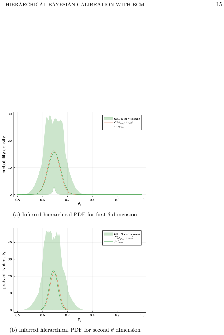
The central claim, argued through benchmark functions and a realistic accelerator case, is that the Bayesian Committee Machine's product-of-experts likelihood can be embedded inside hierarchical Kennedy–O'Hagan calibration without changing the distribution that MCMC samples. The simulation data is split into $N_{\mathrm{MBC}}$ subsets; each subset is combined with the experimental data to form a Gaussian-process likelihood for the trial parameters, and the subset likelihoods are multiplied together and divided by the $(N_{\mathrm{MBC}}-1)$-th power of the Gaussian-process prior so the variance is not underestimated (Equation 2.13). The hierarchical layer draws each experiment's parameter $\theta_i$ from $\mathcal{N}(\mu_\theta, \sigma_\theta)$, so the posterior yields both per-experiment values and the ensemble distribution; the paper shows that the recovered distribution matches the true generating distribution's moments and covariance on all three test problems, including a 2,400-run simulation set for an accelerator electron gun whose field amplitude must be inferred separately for each experiment. From this the paper concludes that the BCM delivers substantial computational gains while preserving inferential accuracy, and that because it partitions data rather than fitting an inducing-point or low-rank approximation, it avoids biases such approximations can introduce.
Load-bearing premise
The posterior in Equation 2.7 treats each experiment's measured output as its own independent Gaussian-process likelihood factor, discarding the correlations among experimental outputs that the joint covariance matrix in Equation 2.11 encodes; if those cross-experiment correlations carry information, the sampled posterior is misspecified and the reported per-experiment uncertainties are not strictly valid.
Editorial extensions
If this is right
- With eight committee members instead of one, the reported runtime speed-up reaches 15.86× at 150 simulation points and the scaling exponent drops from $O(n^{2.31})$ to $O(n^{1.24})$, so doubling the committee roughly allows doubling the simulation set at the same expected cost.
- The hierarchical layer recovers the ensemble distribution of the calibration parameters rather than a pooled mean: the inferred $\mu_\theta$ and $\sigma_\theta$ match the generating distribution's moments on the Park and accelerator examples, and the two-dimensional cantilever case additionally recovers the covariance structure between parameter dimensions.
- Accuracy is preserved only when each committee member sees enough data: the paper finds the error on the inferred moments grows when subsets fall below about 20 simulation points, setting a practical floor on how finely to split.
- Calibration runtime drops from roughly an hour to about five minutes in the demonstrated regime, which is the difference between an offline analysis and an update an accelerator operator can run between measurements.
- The BCM partition approach keeps all simulation points in use rather than selecting a subset, so larger training sets reduce the emulator error without a proportional runtime penalty once the committee structure absorbs the extra points.
Reading between the lines
- The factorization in Equation 2.7 (a product over experiments of univariate Gaussian-process densities) is never flagged in the paper as an approximation, yet it omits the cross-experiment correlations present in the joint covariance of Equation 2.11; if those correlations are informative, the per-experiment uncertainties and the recovered $\sigma_\theta$ could be biased, and an exact-likelihood r
- The paper itself concedes (Section 2.4.1) that the BCM has no proven convergence guarantees outside a small-query regime and that dependence between committee members can distort uncertainty estimates; since the accuracy results are empirical, a conservative transfer rule for new applications is to validate against the full-GP calibration on a subset of the data and to keep each committee member a
- The same product-of-experts construction should transfer to any inverse problem that repeatedly evaluates a Gaussian-process likelihood against a large, splittable simulation set, such as other accelerator components or physics simulations with expensive forward models, because nothing in the derivation is specific to beam physics.
- Replacing the random split with a domain-informed partition and replacing the fixed Gaussian hierarchical density with a heavier-tailed or mixture family would directly address the two acknowledged sources of bias—committee dependence and parametric misspecification of the ensemble distribution—that the paper flags in Sections 2.4.2 and 4.
Signed reviews
Editorial analysis
A structured set of objections, weighed in public.
Referee Report
Summary. The manuscript proposes a hierarchical extension of Kennedy-O'Hagan Bayesian calibration in which each experiment has its own calibration parameter theta_i with a hierarchical prior, and uses the Bayesian Committee Machine to split the simulation dataset for scalable Gaussian-process likelihood evaluation inside NUTS-based MCMC. The method is tested on the Park and cantilever beam benchmarks and on a synthetic Argonne Wakefield Accelerator example. The central claim is that the BCM integration yields substantial runtime savings while preserving inferential accuracy.
Significance. The combination of hierarchical calibration with BCM is a natural and potentially useful contribution for simulation-heavy calibration problems, and the paper provides a concrete Julia implementation, runtime scaling experiments, and an honest discussion of BCM limitations. However, the manuscript's accuracy claims are undermined by an internal inconsistency in the likelihood definition and by a direct contradiction in the reported application results, so the significance as presented is not established.
major comments (3)
- [§2.2, Eq. (2.7) and Eq. (2.11)] Equation (2.7) writes the posterior as a product over experiments of univariate GP densities p_GPz(z_exp,i | ...), while Equation (2.11) gives the joint multivariate normal density with covariance K_h(theta, phi). These are not equivalent: after integrating out the shared emulator eta and discrepancy delta, the experimental outputs are correlated through the off-diagonal terms of K_h, and the product in Eq. (2.7) ignores those correlations. The manuscript never identifies Eq. (2.7) as an approximation. If the implementation follows Eq. (2.7), the sampled posterior is based on a misspecified likelihood; if it follows Eq. (2.11), the paper misstates the model. Either way, the claim in §5 that the framework 'quantify[ies] uncertainty reliably' is not supported.
- [§3.6, Table 6] The text states that 'the true value lies within the standard deviation of the corresponding NUTS-MC chain.' This is contradicted by the table in many rows; for example, row 5 has D_exp = 57.5829, E[theta] = 53.8301, and Sigma = 0.0284, a discrepancy of roughly 132 posterior standard deviations, and rows 2, 6, 9, 11, 12, 13, and 14 show similar departures. These results indicate that the individual calibration parameters are not recovered and that the reported posterior uncertainties are far too small, consistent with the misspecification in Eq. (2.7). The accuracy half of the central claim is therefore empirically contradicted by the paper's own application.
- [§2.4.1 and §4] Section 2.4.1 concedes that there are no convergence guarantees for BCM when the number of query points (here, the number of experiments) is below the effective degrees of freedom, and §4 acknowledges that the approximation error has no known bounds. Nevertheless, §4 concludes that 'the BCM approximation is accurate and samples the same target distribution.' That conclusion rests on two benchmarks with particular data ratios and does not cover the AWA regime with N_exp = 15; together with the likelihood inconsistency above, the general claim of 'preserving inferential accuracy' is not established.
minor comments (5)
- [Eq. (2.2)] Equation (2.2) contains rendering artifacts ('radicaltp/radicalvertex') and should be typeset properly.
- [§2.4, after Eq. (2.14)] The discussion after Eq. (2.14) is confusing: it says D_exp is 'not conditionally independent from itself,' but the equation concerns splitting D_sim; please clarify the conditional-independence assumptions in the BCM combination.
- [§2.5] Section 2.5 states that emulator hyperparameters Phi_eta are optimised beforehand, whereas the posterior in Eq. (2.5) includes all hyperparameters; the change in inferential target should be stated explicitly when the model is introduced.
- [Table 6] Table 6 would be clearer if the columns used sigma instead of Sigma for the chain standard deviation, and if the number of committee members used in the AWA run were reported.
- [§3.5] The statement that chain convergence was 'not explicitly evaluated' should be addressed with standard diagnostics such as R-hat, especially since the AWA chains are short.
Circularity Check
No significant circularity: the hierarchical KOH/BCM derivation is built from Bayes' rule and standard GP machinery, hyperparameters are fit to simulation data via empirical Bayes, and all accuracy claims are checked against full-GP benchmarks and true synthetic parameters rather than being read back from the fit.
full rationale
The paper's derivation chain is self-contained and does not reduce a claimed prediction to its own inputs. The posterior in Eq. 2.5 is a direct consequence of Bayes' rule applied to the KOH GP likelihood in Eq. 2.4; the hierarchical extension in Eqs. 2.7-2.10 adds a hierarchical prior on experiment-specific parameters without defining the target distribution in terms of the fitted values. The BCM approximation in Eq. 2.13 is cited to Tresp (exogenous literature, not the authors' prior work) and is used only as a computational approximation of the GP likelihood, whose accuracy is separately checked against the 1-MBC full-GP case on Park, cantilever-beam, and AWA synthetic benchmarks. The pre-optimisation of the simulation-emulator hyperparameters on Dsim (Section 2.5) is empirical Bayes: it fits nuisance hyperparameters to the simulation data, but the calibrated objects of interest are the experiment-specific parameters theta_i and the hierarchical moments, which are not the fitted constants. The paper also discloses the relevant limitations, including the lack of BCM convergence guarantees (Section 2.4.1) and the bias from prescribing a parametric hierarchical distribution (Section 4), which cuts against any attempt to hide a circular premise. A separate correctness concern exists: Eq. 2.7 factors the experimental likelihood into a product over experiments of univariate GP densities while Eq. 2.11 presents the joint multivariate-normal density, and these are not equivalent; Table 6 also shows several Dexp values several posterior standard deviations from the chain means. Those are potential model-misspecification or implementation-validity issues, not instances of a prediction being equivalent by construction to a fitted input. Thus no circularity step meeting the required evidence standard is present.
Assumptions & free parameters
free parameters (1)
- GP emulator hyperparameters (λη, lη) =
not reported in paper
assumptions (5)
- domain assumption BCM conditional independence of simulation subsets Dsim^(i)
- ad hoc to paper Experimental likelihood factorizes as a product of univariate GP marginals (Eq 2.7)
- domain assumption Hierarchical prior θ_i ~ N(µθ, σθ) with uniform hyperpriors
- domain assumption Matérn-3/2 kernel with ARD lengthscales as the emulator covariance
- domain assumption Simulator outputs (OPAL) are the ground truth for synthetic observations
Cite this review
Pith. "Pith review of Hierarchical Bayesian Calibration with Bayesian Committee Machine." pith.science (2026). https://pith.science/paper/GLODGQF4
@misc{pith2026260812603,
  author       = {Pith},
  title        = {Pith review of: Hierarchical Bayesian Calibration with Bayesian Committee Machine},
  year         = {2026},
  howpublished = {\url{https://pith.science/paper/GLODGQF4}},
  note         = {Machine review of arXiv:2608.12603}
}
read the original abstract
Calibrating computational models to experimental data is a core task in applied statistics, especially in scientific domains, where physical experiments are costly and simulations play a central role in design and inference. Motivated by uncertainty quantification challenges in particle accelerator experiments, we develop and evaluate a Hierarchical Bayesian Calibration framework. In contrast to standard Bayesian calibration, certain inputs - such as beam injection amplitude - must be estimated separately for each experiment. We adopt the Kennedy-O'Hagan formulation and extend it with a hierarchical prior structure to model the distribution of experiment-specific calibration parameters, thus borrowing strength and improving generalisation across repeated experiments. A key methodological challenge arises from the need to evaluate a large number of forward simulations, which renders conventional Markov chain Monte Carlo approaches computationally prohibitive. To address this, we leverage the Bayesian Committee Machine as a scalable modelling strategy for Gaussian Process emulators. The BCM provides a principled divide-and-conquer approach, enabling parallel inference and reducing computational cost without requiring problem-specific tuning of the emulator approximation. Posterior sampling is performed using the No-U-Turn Sampler, supported by automatic differentiation in Julia, which removes the need for analytic gradient derivation and facilitates flexible model specification. We assess the proposed framework using established benchmark problems and simulated data from the Argonne Wakefield Accelerator. The results demonstrate substantial computational savings and robust calibration performance, highlighting the applicability of the method to large-scale scientific modelling problems.
Figures


Figures from the paper (10 more)




Reference graph
Works this paper leans on
-
[1]
Bayesian Inference: An Introduction to Principles and Practice in Machine Learning
Tipping ME. Bayesian Inference: An Introduction to Principles and Practice in Machine Learning. In: Bousquet O, von Luxburg U, Rätsch G, editors. Advanced Lectures on Machine Learning: ML Summer Schools 2003, Canberra, Australia, February 2 - 14, 2003, Tübingen, Germany, August 4 - 16, 2003, Revised Lectures. Springer; 2004. p. 41–62. A vailable from: htt...
-
[2]
Bayesian calibration of computer models
Kennedy MC, O’Hagan A. Bayesian calibration of computer models. Journal of the Royal Statistical Society: Series B (Sta- tistical Methodology). 2001;63(3):425–464. A vailable from: https://onlinelibrary.wiley.com/doi/abs/10.1111/1467-9868. 00294
-
[3]
Combining Field Data and Computer Simulations for Calibration and Predic- tion
Higdon D, Kennedy M, Cavendish JC, et al. Combining Field Data and Computer Simulations for Calibration and Predic- tion. SIAM Journal on Scientific Computing. 2004;26(2):448–466. A vailable from: https://epubs.siam.org/doi/10.1137/ S1064827503426693
work page 2004
-
[4]
Computer model validation with functional output
Bayarri MJ, Walsh D, Berger JO, et al. Computer model validation with functional output. The Annals of Statis- tics. 2007;35(5):1874–1906. A vailable from: https://projecteuclid.org/journals/annals-of-statistics/volume-35/issue-5/ Computer-model-validation-with-functional-output/10.1214/009053607000000163.full
-
[5]
Bayarri MJ, Berger JO, Kennedy MC, et al. Predicting Vehicle Crashworthiness: Validation of Computer Models for Functional and Hierarchical Data. Journal of the American Statistical Association. 2009;104(487):929–943. A vailable from: https: //doi.org/10.1198/jasa.2009.ap06623
-
[6]
Computer Model Calibration Using High-Dimensional Output
Higdon D, Gattiker J, Williams B, et al. Computer Model Calibration Using High-Dimensional Output. Journal of the American Statistical Association. 2008;103(482):570–583. A vailable from: https://www.jstor.org/stable/27640080
-
[7]
Reified Bayesian modelling and inference for physical systems
Goldstein M, Rougier J. Reified Bayesian modelling and inference for physical systems. Journal of Statistical Planning and In- ference. 2009;139(3):1221–1239. A vailable from: https://www.sciencedirect.com/science/article/pii/S0378375808003303
work page 2009
-
[8]
Bayesian Hierarchical Modeling for Integrating Low-Accuracy and High-Accuracy Experiments
Qian PZG, Wu CFJ. Bayesian Hierarchical Modeling for Integrating Low-Accuracy and High-Accuracy Experiments. Tech- nometrics. 2008;50(2):192–204. A vailable from: https://www.jstor.org/stable/25471459. This manuscript is for review purposes only. HIERARCHICAL BAYESIAN CALIBRATION WITH BCM 25
Show all 36 references
-
[9]
Efficient calibration for imperfect computer models
Tuo R, Wu CFJ. Efficient calibration for imperfect computer models. The Annals of Statistics. 2015; 43(6):2331–2352. A vailable from: https://projecteuclid.org/journals/annals-of-statistics/volume-43/issue-6/ Efficient-calibration-for-imperfect-computer-models/10.1214/15-AOS1314.full
2015 doi
-
[10]
Bayesian Calibration of Inexact Computer Models
Plumlee M. Bayesian Calibration of Inexact Computer Models. Journal of the American Statistical Association. 2017; 112(519):1274–1285. A vailable from: https://doi.org/10.1080/01621459.2016.1211016
2017
-
[11]
A unified framework for multilevel uncertainty quantification in Bayesian inverse problems
Nagel JB, Sudret B. A unified framework for multilevel uncertainty quantification in Bayesian inverse problems. Prob- abilistic Engineering Mechanics. 2016;43:68–84. A vailable from: https://www.sciencedirect.com/science/article/pii/ S0266892015300266
2016
-
[12]
Gaussian Processes for Machine Learning
Rasmussen CE, Williams CKI. Gaussian Processes for Machine Learning. The MIT Press; 2005. A vailable from: https: //direct.mit.edu/books/oa-monograph/2320/Gaussian-Processes-for-Machine-Learning
2005
-
[13]
Variational Learning of Inducing Variables in Sparse Gaussian Processes
Titsias M. Variational Learning of Inducing Variables in Sparse Gaussian Processes. In: Proceedings of the Twelfth International Conference on Artificial Intelligence and Statistics. PMLR; 2009. p. 567–574. A vailable from: https: //proceedings.mlr.press/v5/titsias09a.html
2009
-
[14]
Convergence of Sparse Variational Inference in Gaussian Processes Regression
Burt DR, Rasmussen CE, van der Wilk M. Convergence of Sparse Variational Inference in Gaussian Processes Regression. Journal of Machine Learning Research. 2020;21(131):1–63. A vailable from: http://jmlr.org/papers/v21/19-1015.html
2020
-
[15]
Adaptive Sparse Variational Approximations for Gaussian Process Regression
Nieman D, Szabó B. Adaptive Sparse Variational Approximations for Gaussian Process Regression. Bayesian Analysis. 2025;:1–20A vailable from: https://projecteuclid.org/journals/bayesian-analysis/advance-publication/ Adaptive-Sparse-Variational-Approximations-for-Gaussian-Proces...
2025 doi
-
[16]
Estimation and Model Identification for Continuous Spatial Processes
Vecchia A V. Estimation and Model Identification for Continuous Spatial Processes. Journal of the Royal Statistical Society Series B (Methodological). 1988;50(2):297–312. A vailable from: https://www.jstor.org/stable/2345768
1988
-
[17]
A General Framework for Vecchia Approximations of Gaussian Processes
Katzfuss M, Guinness J. A General Framework for Vecchia Approximations of Gaussian Processes. Statistical Sci- ence. 2021;36(1):124–141. A vailable from: https://projecteuclid.org/journals/statistical-science/volume-36/issue-1/ A-General-Framework-for-Vecchia-Approximations-of...
2021 doi
-
[18]
Using the Nyström Method to Speed Up Kernel Machines
Williams C, Seeger M. Using the Nyström Method to Speed Up Kernel Machines. In: Advances in Neural Information Processing Systems; Vol. 13. MIT Press; 2000. A vailable from: https://papers.nips.cc/paper_files/paper/2000/hash/ 19de10adbaa1b2ee13f77f679fa1483a-Abstract.html
2000
-
[19]
When Gaussian Process Meets Big Data: A Review of Scalable GPs
Liu H, Ong YS, Shen X, et al. When Gaussian Process Meets Big Data: A Review of Scalable GPs. IEEE Transactions on Neural Networks and Learning Systems. 2020;31(11):4405–4423. A vailable from: https://ieeexplore.ieee.org/document/ 8951257
2020
-
[20]
A Bayesian Committee Machine
Tresp V. A Bayesian Committee Machine. Neural Computation. 2000;12(11):2719–2741. A vailable from: https://direct.mit. edu/neco/article/12/11/2719-2741/6426
2000
-
[21]
Gaussian Processes for Regression
Williams C, Rasmussen C. Gaussian Processes for Regression. In: Advances in Neural Information Pro- cessing Systems; Vol. 8. MIT Press; 1995. A vailable from: https://proceedings.neurips.cc/paper/1995/hash/ 7cce53cf90577442771720a370c3c723-Abstract.html
1995
-
[22]
Prior distributions for variance parameters in hierarchical models (comment on article by Browne and Draper)
Gelman A. Prior distributions for variance parameters in hierarchical models (comment on article by Browne and Draper). Bayesian Analysis. 2006;1(3):515–534. A vailable from: https://projecteuclid.org/journals/bayesian-analysis/volume-1/ issue-3/Prior-distributions-for-varianc...
2006 doi
-
[23]
Generating random correlation matrices based on vines and extended onion method
Lewandowski D, Kurowicka D, Joe H. Generating random correlation matrices based on vines and extended onion method. Journal of Multivariate Analysis. 2009;100(9):1989–2001. A vailable from: https://www.sciencedirect.com/science/article/ pii/S0047259X09000876
2009
-
[24]
The No-U-Turn Sampler: Adaptively Setting Path Lengths in Hamiltonian Monte Carlo
Hoffman MD, Gelman A. The No-U-Turn Sampler: Adaptively Setting Path Lengths in Hamiltonian Monte Carlo. Journal of Machine Learning Research. 2014;15(47):1593–1623. A vailable from: http://jmlr.org/papers/v15/hoffman14a.html
2014
-
[25]
Turing: A Language for Flexible Probabilistic Inference
Ge H, Xu K, Ghahramani Z. Turing: A Language for Flexible Probabilistic Inference. In: Proceedings of the Twenty-First International Conference on Artificial Intelligence and Statistics. PMLR; 2018. p. 1682–1690. A vailable from: https: //proceedings.mlr.press/v84/ge18b.html
2018
-
[26]
AdvancedHMC.jl: A robust, modular and efficient implementation of advanced HMC algo- rithms
Xu K, Ge H, Tebbutt W, et al. AdvancedHMC.jl: A robust, modular and efficient implementation of advanced HMC algo- rithms. In: Proceedings of The 2nd Symposium on Advances in Approximate Bayesian Inference. PMLR; 2020. p. 1–10. A vailable from: https://proceedings.mlr.press/v11...
2020
-
[27]
Sparse Greedy Gaussian Process Regression
Smola A, Bartlett P. Sparse Greedy Gaussian Process Regression. In: Advances in Neural Information Process- ing Systems; Vol. 13. MIT Press; 2000. A vailable from: https://papers.nips.cc/paper_files/paper/2000/hash/ 3214a6d842cc69597f9edf26df552e43-Abstract.html
2000
-
[28]
Fast Sparse Gaussian Process Methods: The Informative Vector Machine
Lawrence N, Seeger M, Herbrich R. Fast Sparse Gaussian Process Methods: The Informative Vector Machine. In: Advances in Neural Information Processing Systems; Vol. 15. MIT Press; 2002. A vailable from: https://papers.nips.cc/paper_files/ paper/2002/hash/d4dd111a4fd973394238aca...
2002
-
[29]
Distributed Gaussian processes
Deisenroth MP, Ng JW. Distributed Gaussian processes. In: Proceedings of the 32nd International Conference on Machine Learning - Volume 37; (ICML’15; Vol. 37). JMLR.org; 2015. p. 1481–1490
2015
-
[30]
Sparse On-Line Gaussian Processes
Csató L, Opper M. Sparse On-Line Gaussian Processes. Neural Computation. 2002;14(3):641–668. A vailable from: https: //doi.org/10.1162/089976602317250933
2002 doi
-
[31]
Generalized Robust Bayesian Committee Machine for Large-scale Gaussian Process Regression
Liu H, Cai J, Wang Y, et al. Generalized Robust Bayesian Committee Machine for Large-scale Gaussian Process Regression. In: Proceedings of the 35th International Conference on Machine Learning. PMLR; 2018. p. 3131–3140. A vailable from: https://proceedings.mlr.press/v80/liu18a.html
2018
-
[32]
A sparse Bayesian Committee Machine potential for oxygen-containing organic compounds
Willow SY, Kim S, Yang DC, et al. A sparse Bayesian Committee Machine potential for oxygen-containing organic compounds. Chemical Physics Reviews. 2025;6(2). A vailable from: https://pubs.aip.org/aip/cpr/article/6/2/021401/ 3344282/A-sparse-Bayesian-Committee-Machine-potential-for
2025
-
[33]
A statistical method for tuning a computer code to a data base
Cox DD, Park JS, Singer CE. A statistical method for tuning a computer code to a data base. Computational Statistics & Data Analysis. 2001;37(1):77–92. A vailable from: https://www.sciencedirect.com/science/article/pii/S0167947300000578
2001
-
[34]
Investigation of reliability method formulations in DAKOTA/UQ
Eldred MS, Agarwal H, Perez VM, et al. Investigation of reliability method formulations in DAKOTA/UQ. Structure and Infrastructure Engineering. 2007;3(3):199–213. A vailable from: https://doi.org/10.1080/15732470500254618
2007 doi
-
[35]
Research Program and Recent Results at the Argonne Wakefield Accelerator Facility (A W A)
Conde M, Antipov S, Doran D, et al. Research Program and Recent Results at the Argonne Wakefield Accelerator Facility (A W A). JACOW, Geneva, Switzerland; 2017. p. 2885–2887. A vailable from:https://proceedings.jacow.org/ipac2017/doi/ JACoW-IPAC2017-WEPAB132.html
2017
-
[36]
OPAL a Versatile Tool for Charged Particle Accelerator Simulations; 2019
Adelmann A, Calvo P, Frey M, et al. OPAL a Versatile Tool for Charged Particle Accelerator Simulations; 2019. A vailable from: http://arxiv.org/abs/1905.06654. This manuscript is for review purposes only
2019 arXiv
Reviewed August 16, 2026 · model on record in the stance chip above.
Discussion (0). Continue with ORCID to comment.