How Loud Must a Neutron-Star Merger Be to Reveal Its Equation of State?

Sk Md Adil Imam

REVIEW 3 major objections 5 minor 35 references

How Loud Must a Neutron-Star Merger Be to Reveal Its Equation of State?

T0 review · 3 major / 5 minor · reviewed 2026-08-07 · deepseek-v4-flash

Challenge this review Re-run · record.json Download PDF Read on arXiv ↗

Pith's one-line read For zero-noise binary neutron-star signals in a third-generation detector network, the Bayesian evidence ratio between competing equations of state follows $\Delta\log Z \approx C\,(\Delta\tilde{\Lambda}\,\mathrm{SNR})^2$, with a…

desk verdict Useful, honest empirical study of EOS-discrimination SNR, but the signature 0.3% transfer claim rests on a single draw and a prefactor calibrated at SNR~3355 being applied at SNR~50. read the letter →

arxiv 2608.05794 v1 pith:2DKAHUZN submitted 2026-08-06 gr-qc

Sk Md Adil Imam This is my paper · ORCID

classification gr-qc

keywords neutron-starequationofstatetidaldeformabilitygravitational-waveastronomyBayesianmodelselectionOccamfactorthird-generationdetectorsnestedsamplingSNRthreshold

verification ladder T0 review T1 audit T2 compute T3 formal

The pith

A machine-rendered reading of the paper's core claim, the machinery that carries it, and where it could break.

The reading

This paper tries to show that the loudness threshold at which a single neutron-star merger lets gravitational-wave data choose between two candidate equations of state can be written as a closed-form law rather than measured by expensive simulations. Across four configurations that vary the tidal-deformability contrast, the true/wrong EOS role, and the binary mass, the log-evidence difference between the correct and incorrect recovery model follows $\Delta\log Z \approx C\,(\Delta\tilde{\Lambda}\,\mathrm{SNR})^2$, with empirical exponents $n\approx 1.74$--$1.95$ trending toward $2$ at high SNR. The prefactor $C$ is fitted from three configurations and then used to predict, before the run, the decisive-evidence SNR of a fourth configuration; the measured value (50.7) agreed with the pre-registered prediction (50.8) within 0.3%. If the scaling is right, event selection for the Einstein Telescope and Cosmic Explorer can be planned with a pencil-and-paper estimate, provided $C$ is recalibrated for each EOS pair and mass regime.

What carries the argument

The key machinery is the Laplace/Occam-factor expansion of the Bayesian evidence, which turns the evidence difference into $\frac{1}{2}\|\delta h_\perp\|^2$, where $\delta h_\perp$ is the noise-weighted waveform mismatch between the correct and wrong-EOS templates after all nuisance parameters (mass ratio, spin, coalescence time) are optimized. Because the wrong-EOS arm can compensate part of the tidal mismatch by shifting these nuisance parameters, only the orthogonalized residual $\delta h_\perp$ contributes to the penalty, and this construction is what carries the argument from waveform mismatch to model selection. At leading post-Newtonian order the tidal phase is linear in $\tilde{\Lambda}$, so the residual mismatch is proportional to $\Delta\tilde{\Lambda}\,\mathrm{SNR}$, giving the closed-form threshold relation $\rho_T = (1/\Delta\tilde{\Lambda})\sqrt{T/C}$ for a Jeffreys-scale label $T$.

What would settle it

Take an EOS pair and a binary mass point that appear in none of the paper's four curves or five spot-checks, calibrate $C$ from three high-SNR anchor runs, and measure the decisive-evidence SNR with full nested sampling; if the measured value falls outside the pre-registered 95% prediction interval, or if the zero-noise $\Delta\log Z$ at a moderate SNR around 40 deviates from $C(\Delta\tilde{\Lambda}\,\mathrm{SNR})^2$ by more than the roughly 30% scatter seen in $C$, the claimed predictive transferability is falsified.

Watch

Extended reading notes

Core claim

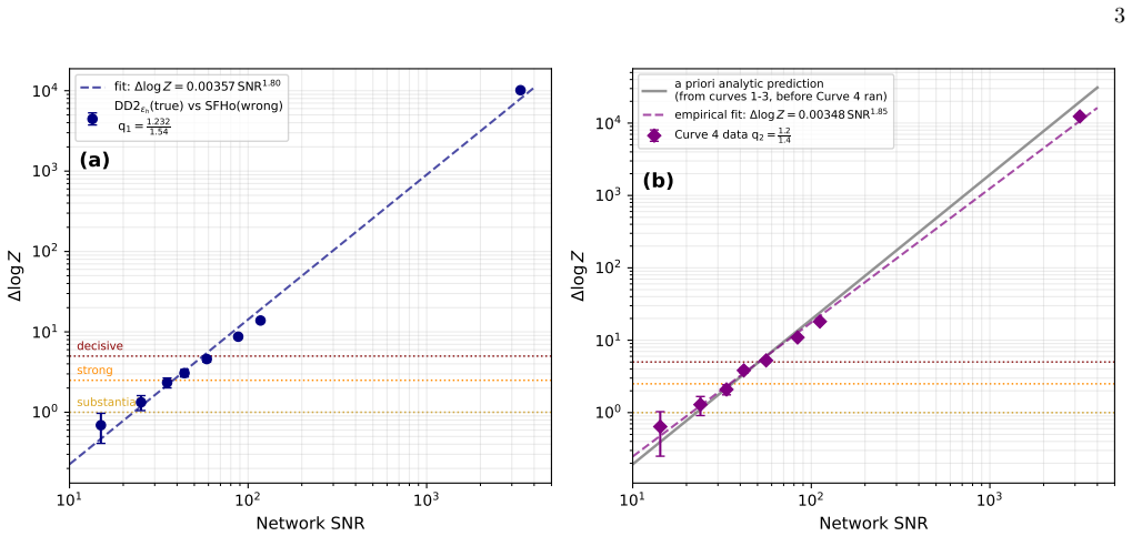
The central claim is that the Occam-factor penalty for recovering a neutron-star signal with the wrong equation of state is, at leading order, half the squared noise-weighted mismatch between the correct and wrong templates, and because the tidal phase is linear in the mass-weighted tidal deformability $\tilde{\Lambda}$, the evidence difference reduces to $\Delta\log Z \approx C\,(\Delta\tilde{\Lambda}\,\mathrm{SNR})^2$. The paper verifies this with full Bayesian nested-sampling parameter estimation on zero-noise simulated signals in an Einstein Telescope plus two Cosmic Explorer network, using the IMRPhenomD NRTidalv2 waveform, and shows that the fitted exponent approaches the asymptotic value 2 as SNR grows. It then demonstrates the relation's predictive power: calibrating the prefactor $C$ from three configurations at an anchor SNR near 3355, it predicted the decisive-evidence SNR for a fourth, independent binary mass point as 50.8, and the subsequent measurement gave 50.7, within the pre-registered 95% interval. The paper stresses that $C$ is not universal — it depends on masses, spins, sky location, and the detector network — and that the exponent statement is best read as a trend toward 2, since dropping the highest-SNR anchor point substantially weakens the constraint on $n$.

Load-bearing premise

The whole predictive scheme rests on the assumption that a prefactor $C$ calibrated at very loud, noise-free signals with a single sky position and inclination transfers unchanged to the moderate-SNR regime and to binary configurations outside the calibration set, where the wrong-EOS arm may compensate the mismatch in different ways.

Editorial extensions

If this is right

For a fixed EOS pair and detector network, the decisive-discrimination SNR can be computed as $(1/\Delta\tilde{\Lambda})\sqrt{5/C}$, turning an expensive nested-sampling campaign into a one-line estimate.
Reducing the tidal-deformability contrast between two candidates pushes all Jeffreys-threshold SNRs upward while leaving the scaling exponent unchanged, and near-degenerate EOS pairs with $\Delta\tilde{\Lambda}\approx 10$--$30$ would require SNR around 900--2800, within reach only for rare, GW170817-distance-like events.
Swapping which EOS is injected and which is recovered changes threshold SNRs by only about 20%, so the scaling is not an artifact of one EOS being the 'true' one.
The exponent $n$ is best interpreted as approaching $2$ as SNR increases rather than as a tightly constrained constant; densifying the high-SNR grid reduces the anchor point's leverage sevenfold, so the quadratic law is supported by continuity of the local slope $K=\Delta\log Z/\mathrm{SNR}^2$.

Reading between the lines

Editorial extensions of the paper, not claims the author makes directly.

A natural extension the paper leaves implicit: the same Occam-factor argument should apply to any discrete model-selection problem where the waveform difference is linear in a scalar parameter, such as choosing among modified-gravity theories, giving an analogous $(\Delta \text{parameter} \times \mathrm{SNR})^2$ law with a redefined prefactor.
The doppelg\"anger caveat suggests that single-event loudness will not settle the equation of state for pairs of physically distinct EOS that nearly agree in $\tilde{\Lambda}$; population-level or multi-messenger information rather than a solitary loud burst would carry that part of the program.
A cheap test of the framework's scope would be to densify the SNR grid for Curves 2--4 the way Curve 1 was densified, checking whether the smooth, curvature-free decline of $K$ seen in Curve 1 generalizes before trusting the high-SNR asymptotic form away from the fiducial configuration.

Share X Bluesky LinkedIn Reddit HN

Editorial analysis

A structured set of objections, weighed in public.

Desk editor's note, referee report, and a circularity audit.

Desk Editor's Note

read the letter

I've been through Imam's paper on the SNR needed to tell two neutron-star EOS apart with 3G detectors. The short version: the empirical study is solid and the author is unusually candid about limitations, but the headline transfer claim is thinner than the 0.3% framing suggests.

What's actually new: a closed-form estimate ΔlogZ ≈ C(ΔΛ·ρ)² derived from an Occam/Laplace argument, calibrated on three zero-noise configurations and used to predict a fourth configuration's decisive-evidence SNR before running it. That's a genuine pre-registered out-of-sample test, and the data and code are public. Four of five spot-checks across other EOS pairs transfer within ~15%. The author also flags his own soft spots—anchor leverage, an unidentified ~3σ excess between Curves 1 and 3 in the SNR 25–60 range, prior-boundary pinning, and one spot-check that lands at 44% of the prediction. That honesty earns credit.

The soft spot is load-bearing. The measured power-law exponents are n≈1.8, not 2. That means the effective coefficient C_eff = ΔlogZ/(ΔΛ·ρ)² is not constant across SNR; it changes by roughly a factor of 1.5–2 between the calibration anchor (SNR≈3355) and the threshold region (SNR≈20–90). The 95% prediction interval in Table S2 only includes the calibration scatter in C, not this scale-extrapolation error, so the uncertainty is understated. The Curve 4 agreement (50.7 vs 50.8) is a single draw in which Curve 4's moderate-SNR C_eff happened to sit near the calibration mean; Curve 4's own anchor coefficient is actually an outlier by a similar factor. That doesn't validate the quadratic law across the range.

The author himself says C is not universal and needs recalibration, and the densification runs show the anchor-leverage was partly a sparse-sampling artifact. So the framework is worth having as a planning tool, but the abstract's 'within 0.3%' is a precision claim the analysis doesn't actually support.

Who is this for: anyone making 3G sensitivity forecasts for EOS discrimination. It deserves a serious referee. In revision, the author should either validate C with runs at moderate SNR or quote a wider uncertainty that includes the n<2 drift; and the Curve 1/3 discrepancy should be chased down. I'd send it to review.

Referee Report

3 major / 5 minor

Summary. The paper performs full Bayesian nested-sampling parameter estimation on simulated binary neutron star signals in an ET+2CE network, using zero-noise injections and the IMRPhenomD NRTidalv2 waveform, and measures the log-evidence difference between a correct-EOS and an incorrect-EOS recovery model across four configurations and a range of network SNR. The central claim is that this difference follows a near-quadratic scaling, ΔlogZ ≈ C(ΔΛ̃·SNR)^2, with C dependent on binary properties and detector configuration but transferable across configurations once calibrated. The headline quantitative test is a pre-registered, out-of-sample prediction: calibrating C on three configurations at the dL=42 Mpc anchor (SNR≈3355) predicts a decisive-evidence threshold for a fourth, unmeasured binary mass point at SNR≈50.8, and the subsequently measured value is 50.7, inside the pre-registered 95% interval. The paper also reports a five-draw spot-check across further EOS pairs in which four of five draws agree within ~15%, with one 44% underprediction attributed to unusually efficient mass-ratio compensation.

Significance. If the scaling law and the transferability of C were robust, the paper would provide a practical planning tool for 3G detectors and a useful bridge between analytic Occam-factor arguments and full Bayesian model selection. The paper is commendably transparent: it includes an explicit derivation of the leading-order quadratic form, a genuine out-of-sample pre-registered test, per-point data tables, anchor-leverage sensitivity analyses, a densification check, a free-sky/noise robustness check, and public code and data. These are real strengths. However, the load-bearing extrapolation from the anchor SNR to the moderate-SNR threshold regime is not supported by the paper's own data: within a single curve the effective coefficient ΔlogZ/(ΔΛ̃^2 SNR^2) varies by up to a factor of ~1.8 between the anchor and the decisive threshold, and the anchor-dropped fits in the threshold regime give exponents as low as n=1.20-1.75. The Curve 4 prediction therefore rests on an unquantified scale extrapolation, and the 0.3% agreement, while striking, is a single draw rather than evidence that the anchor calibration constrains the prediction regime.

major comments (3)

[Supplemental Material, 'Derivation of the analytic scaling relation', Eq. (4), Tables S3 and S7] The coefficient in the claimed quadratic law is not constant across SNR within a single curve. For Curve 1, K = ΔlogZ/SNR^2 decreases monotonically from 3.07e-3 at SNR=14.99 to 9.01e-4 at the SNR=3355 anchor, a factor of 3.4. Equivalently, the effective coefficient C_eff = K/(ΔΛ̃)^2 at the Curve 1 decisive threshold (SNR=55.9) is about 1.09e-8, while the anchor value in Table S1 is 6.18e-9; using the anchor value alone would predict a decisive threshold of ~74.5 instead of the measured 55.9. The Curve 4 prediction in Table S2 is made at SNR≈50 using C calibrated at SNR≈3355, and the reported 95% interval propagates only the ±12.9% anchor-to-anchor scatter, not this scale dependence. The 0.3% agreement at the Curve 4 decisive threshold is therefore a single draw and cannot by itself validate the quadratic law in the prediction regime.
[Table S8 and 'Curve 1 densification' subsection] The anchor-drop sensitivity analysis directly exposes the problem. Removing the anchor lowers the fitted exponent to n=1.20-1.75, and the remaining seven points per curve span only SNR≈15-117, which is exactly the regime where the decisive thresholds for Curves 1-4 lie. The densification of Curve 1 fills the gap between SNR≈117 and SNR≈3355 and shows smooth behavior there, but it contains no point below SNR≈117; hence it does not constrain K in the regime where the predictions are made. The statement that the fitted exponent 'trends toward' the asymptotic n=2 is therefore not supported in the moderate-SNR regime that matters for the headline prediction.
[Table S9, SLy4/FSU2 spot-check] The spot-check campaign provides a direct counterexample to the transferability claim in the prediction regime. For SLy4(true)/FSU2(wrong) at m1/m2=1.8/1.2, the Bayesian inference gives ΔlogZ=1.11±0.32 against the analytical prediction of 2.50, i.e., only 44% of the predicted value, at SNR≈43. The paper attributes this to unusually efficient mass-ratio compensation and notes that the same EOS pair at a different mass ratio does not show the suppression. This is an honest and informative caveat, but it also demonstrates that the scaling estimate can fail by more than a factor of two in the exact SNR regime where the paper wants to predict thresholds. The conclusion should be reframed so that the 'closed-form estimate' is presented as a rough first-order benchmark requiring per-configuration recalibration, not as a predictive law validated by the Curve 4 result.

minor comments (5)

[Abstract and Table I] The abstract states n≃1.74-1.95 while the main text variously says n≈1.8-2 and n=1.74-1.95; please unify the quoted range in the abstract, conclusion, and Table I.
[Eq. (3)] In Eq. (3), the integral J is defined with an integrand containing Sn(f), but Sn(f) is not defined at that point; please specify that it is the one-sided noise power spectral density of the network and state the convention used.
[Figure S2 caption] The caption reads '15 off normal incidence'; this should be '15° off normal incidence' with the degree symbol.
[Supplemental Material, 'Bayesian inference setup'] The phrase 'A point easily missed: Λ1 and Λ2 are not themselves free sampled parameters' is useful but phrased informally; consider moving this explanation to a dedicated paragraph or figure caption so it reads as a standard methodological note.
[Table S9 column definitions] The definitions of 'Analytical', 'Fit', and 'Fit (n=2)' are dense and appear partially after the table; please move them into the table caption or a clear preceding paragraph so the columns are self-explanatory.

Circularity Check

0 steps flagged · score 0.0 of 10

No significant circularity: the quadratic scaling is derived from a Laplace/Occam expansion, and the Curve 4 prediction uses a prefactor calibrated on three separate configurations, not on the predicted configuration.

full rationale

The paper's derivation chain is self-contained. The central scaling ΔlogZ ≈ C(ΔΛ̃·SNR)^2 is obtained in the Supplemental Material by a Laplace/Occam-factor expansion of the evidence, with C defined as I⊥/2, a distance-independent integral, rather than taken from a fit to the predicted configuration. The prefactor is calibrated from the anchor points of Curves 1–3 (Table S1) and then used to predict the decisive-evidence SNR for Curve 4, a binary mass point that was not part of the calibration set; the reported empirical threshold came from an independent nested-sampling run (Tables S6 and S8). No equation in the paper reduces the Curve 4 prediction to a fitted value of Curve 4 itself. The only self-references are to the publicly available code and data repositories [27,28], which are not load-bearing for the physical claim. The paper explicitly discloses the anchor-leverage sensitivity of the fitted exponent and the moderate-SNR scatter in C; these are correctness or extrapolation caveats, not circularity, and the manuscript does not conceal them.

Assumptions & free parameters 4 free parameters · 6 assumptions · 0 invented entities

The central scaling law is derived from a Laplace or Occam expansion with two leading-order truncations: a linear tidal phase in Lambda and neglect of the posterior-volume term Delta vol. The prefactor C is measured from anchor-point evidence, not derived. The paper's key added assumption is that C transfers from extreme SNR to threshold SNR and across mass and EOS pairs; the Curve 4 test and five spot checks provide direct evidence for this in the tested cases. No new physical entities are introduced.

free parameters (4)

Prefactor C = 7.19e-9 (mean of Curves 1-3)
Calibration constant in Delta log Z approximately C times (Delta Lambda times SNR) squared; measured from the anchor point (d_L = 42 Mpc, SNR about 3355) of three configurations and used for the out-of-sample Curve 4 prediction.
Power-law exponent n = 1.74-1.95 per curve; 1.20-1.75 without the anchor point
Empirically fitted exponent in Delta log Z = A times SNR to the n. It is presented as trending toward the asymptotic Occam-factor value n = 2, but is anchor-dependent.
Power-law amplitude A = 3.57e-3, 2.08e-3, 1.46e-3, 3.48e-3 per curve
Fitted normalization for each of the four curves; encodes the EOS contrast and binary properties in the empirical power law.
Hybrid EOS transition energy density epsilon_t = 500 and 200 MeV fm^-3 (epsilon_h and epsilon_l)
Hand-chosen to construct the fiducial DD2 epsilon_h and near-degenerate DD2 epsilon_l models; sets the tidal-deformability contrast used in Curve 2.

assumptions (6)

standard math The Bayesian evidence integral can be approximated by a Laplace expansion about the best fit.
Used in the Supplemental Material derivation of Delta log Z approximately one half of the squared mismatch norm; it is asymptotically valid at high SNR and is tested at moderate SNR by the data.
domain assumption To leading post-Newtonian order, the tidal waveform phase is linear in the mass-weighted tidal deformability Lambda.
In the derivation, delta Psi_perp approximately Delta Lambda times g1(f); higher-order tidal terms are neglected and contribute to the about 30 percent scatter in C.
ad hoc to paper The posterior-volume and prior terms Delta vol in the evidence difference are subleading and can be dropped or absorbed into the calibration scatter.
The paper explicitly says it does not compute Delta vol analytically; the derivation of the quadratic scaling relies on dropping it. The out-of-sample prediction provides empirical support.
domain assumption Zero-noise injections make the noise cross-term vanish and enforce log L(theta_true) = 0.5 SNR squared exactly.
Used in the Method and in Eq. (2); all main-grid runs use zero detector noise, with one free-sky real-noise robustness check at a single point.
domain assumption The prefactor C, calibrated at extreme SNR, transfers to moderate SNR and across binary mass and EOS pairs.
The paper warns that C is not universal and requires recalibration; the Curve 4 test and five spot checks are the evidence for limited transferability.
domain assumption The IMRPhenomD NRTidalv2 waveform and the EOS mass-Lambda tables adequately represent tidal effects for EOS discrimination.
Both injection and recovery use the same waveform model, so internal consistency is guaranteed; realism for actual detections depends on waveform fidelity.

how reviews work

0 comments

Cite this review

Pith. "Pith review of How Loud Must a Neutron-Star Merger Be to Reveal Its Equation of State?." pith.science (2026). https://pith.science/paper/2DKAHUZN

@misc{pith2026260805794,
  author       = {Pith},
  title        = {Pith review of: How Loud Must a Neutron-Star Merger Be to Reveal Its Equation of State?},
  year         = {2026},
  howpublished = {\url{https://pith.science/paper/2DKAHUZN}},
  note         = {Machine review of arXiv:2608.05794}
}

abstract

The tidal response of neutron stars during binary inspiral encodes the equation of state (EOS) of dense matter in the gravitational-wave signal. Quantifying the signal-to-noise ratio (SNR) required to distinguish competing EOS models with third-generation detectors is therefore essential. We perform Bayesian nested-sampling parameter estimation on simulated binary neutron star signals observed by an Einstein Telescope plus two Cosmic Explorer detector network and compute the evidence difference between correct- and incorrect-EOS recovery models over a broad range of SNR. Across two tidal-deformability contrasts, a swap of the true and recovery EOS, and two binary mass points, we find a common scaling, $\Delta\log Z = A\,\mathrm{SNR}^{n}$ with $n \simeq 1.74$--$1.95$, where the EOS contrast and binary properties determine only the prefactor $A$. This behavior follows from an Occam-factor argument, yielding $\Delta\log Z \propto (\Delta\tilde{\Lambda}\,\mathrm{SNR})^{2}$. Calibrating this relation on three configurations predicts, before the run, the SNR required for decisive EOS discrimination in the fourth to within $0.3\%$. These results establish a quantitative framework for assessing the EOS-discrimination reach of third-generation gravitational-wave detector networks.

Figures

Figures reproduced from arXiv: 2608.05794 by the authors.

Discussion (0). Continue with ORCID to comment.

Reference graph

Works this paper leans on

35 extracted references · 11 canonical work pages

[1]

J. S. Read, L. Baiotti, J. D. E. Creighton, J. L. Friedman, B. Giacomazzo, K. Kyutoku, C. Markakis, L. Rezzolla, M. Shibata, and K. Taniguchi, Phys. Rev. D88, 044042 (2013), arXiv:1306.4065

arXiv 2013
[2]

B. P. Abbottet al.(LIGO Scientific, Virgo), Phys. Rev. Lett.119, 161101 (2017), arXiv:1710.05832 [gr-qc]

arXiv 2017
[3]

Punturoet al., Class

M. Punturoet al., Class. Quant. Grav.27, 194002 (2010)

2010
[4]

Reitzeet al., Bull

D. Reitzeet al., Bull. Am. Astron. Soc.51, 035 (2019), arXiv:1907.04833 [astro-ph.IM]

arXiv 2019
[5]

Measuring tidal effects with the Einstein Telescope: A design study

A. Puecher, A. Samajdar, and T. Dietrich, Phys. Rev. D108, 023018 (2023), arXiv:2304.05349 [astro-ph.IM]

work page Pith review arXiv 2023
[6]

L. Wade, J. D. E. Creighton, E. Ochsner, B. D. Lackey, B. F. Farr, T. B. Littenberg, and V. Raymond, Phys. Rev. D89, 103012 (2014)

work page 2014
[7]

B. D. Lackey and L. Wade, Phys. Rev. D91, 043002 (2015)

work page 2015
[8]

Kashyap, I

R. Kashyap, I. Gupta, A. Dhani, M. Bapna, and B. Sathyaprakash, Phys. Rev. D113, 063019 (2026), arXiv:2502.03831 [gr-qc]

work page arXiv 2026

Show all 35 references

[9]

Biswas, E

B. Biswas, E. Smyrniotis, I. Liodis, and N. Stergioulas, Phys. Rev. D109, 064048 (2024), arXiv:2309.05420

2024 arXiv
[10]

B. P. Abbottet al.(LIGO Scientific, Virgo), Class. Quant. Grav.37, 045006 (2020), arXiv:1908.01012 [gr-qc]

2020 arXiv
[11]

Lindblom, B

L. Lindblom, B. J. Owen, and D. A. Brown, Phys. Rev. D78, 124020 (2008), arXiv:0809.3844 [gr-qc]

2008 arXiv
[12]

T. D. P. Edwards, K. W. K. Wong, K. K. H. Lam, A. Coogan, D. Foreman-Mackey, M. Isi, and A. Zimmerman, Phys. Rev. D110, 064028 (2024), arXiv:2302.05329 [astro-ph.IM]

2024 arXiv
[13]

K. W. K. Wong, M. Isi, and T. D. P. Edwards, Astrophys. J.958, 129 (2023), arXiv:2302.05333 [astro-ph.IM]

2023 arXiv
[14]

Wouters, P

T. Wouters, P. T. H. Pang, T. Dietrich, and C. Van Den Broeck, Phys. Rev. D110, 083033 (2024), arXiv:2404.11397 [astro-ph.IM]

2024
[15]

Dietrich, S

T. Dietrich, S. Bernuzzi, and W. Tichy, Phys. Rev. D96, 121501 (2017), arXiv:1706.02969 [gr-qc]

2017 arXiv
[16]

Dietrich, A

T. Dietrich, A. Samajdar, S. Khan, N. K. Johnson-McDaniel, R. Dudi, and W. Tichy, Phys. Rev. D100, 044003 (2019), arXiv:1905.06011 [gr-qc]

2019 arXiv
[17]

J. R. Oppenheimer and G. M. Volkoff, Phys. Rev.55, 374 (1939)

1939
[18]

R. C. Tolman, Phys. Rev.55, 364 (1939)

1939
[19]

A. W. Steiner, M. Hempel, and T. Fischer, Astrophys. J.774, 17 (2013)

2013
[20]

Typel, G

S. Typel, G. R¨ opke, T. Kl¨ ahn, D. Blaschke, and H. H. Wolter, Phys. Rev. C81, 015803 (2010)

2010
[21]

B. P. Abbottet al.(LIGO Scientific, Virgo), Astrophys. J. Lett.848, L12 (2017), arXiv:1710.05833 [astro-ph.HE]. 14

2017 arXiv
[22]

Hotokezaka, E

K. Hotokezaka, E. Nakar, O. Gottlieb, S. Nissanke, K. Masuda, G. Hallinan, K. P. Mooley, and A. T. Deller, Nature Astron.3, 940 (2019), arXiv:1806.10596

2019 arXiv
[23]

Jeffreys,Theory of Probability, 3rd ed

H. Jeffreys,Theory of Probability, 3rd ed. (Oxford University Press, Oxford, 1961)

1961
[24]

Chabanat, P

E. Chabanat, P. Bonche, P. Haensel, J. Meyer, and R. Schaeffer, Nucl. Phys. A635, 231 (1998), [Erratum: Nucl.Phys.A 643, 441–441 (1998)]

1998
[25]

C. A. Raithel and E. R. Most, Phys. Rev. Lett.130, 201403 (2023), arXiv:2208.04294 [astro-ph.HE]

2023 arXiv
[26]

C. A. Raithel and E. R. Most, Phys. Rev. D108, 023010 (2023), arXiv:2208.04295 [astro-ph.HE]

2023 arXiv
[27]

how loud must a neutron-star merger be to reveal its equation of state?

S. M. A. Imam, Jim nested sampling: Code and data for “how loud must a neutron-star merger be to reveal its equation of state?” (2026), GitHub repository. Accessed July 2026

2026
[28]

how loud must a neutron-star merger be to reveal its equation of state?

S. M. A. Imam, Data for “how loud must a neutron-star merger be to reveal its equation of state?”, Zenodo (2026)

2026
[29]

Iacovelli, M

F. Iacovelli, M. Mancarella, S. Foffa, and M. Maggiore, Astrophys. J. Suppl.263, 2 (2022), arXiv:2207.06910

2022 arXiv
[30]

Srivastava, D

V. Srivastava, D. Davis, K. Kuns, P. Landry, S. Ballmer, M. Evans, E. D. Hall, J. Read, and B. S. Sathyaprakash, Astrophys. J.931, 22 (2022), arXiv:2201.10668

2022 arXiv
[31]

Branchesiet al., Journal of Cosmology and Astroparticle Physics2023(07), 068

M. Branchesiet al., Journal of Cosmology and Astroparticle Physics2023(07), 068
[32]

B. P. Abbottet al., Astrophys. J. Lett.848, L13 (2017), arXiv:1710.05834

2017 arXiv
[33]

G. A. Lalazissis, T. Nikˇ si´ c, D. Vretenar, and P. Ring, Phys. Rev. C71, 024312 (2005)

2005
[34]

Chen and J

W.-C. Chen and J. Piekarewicz, Phys. Rev. C90, 044305 (2014)

2014
[35]

G. A. Lalazissis, J. K¨ onig, and P. Ring, Phys. Rev. C55, 540 (1997), arXiv:nucl-th/9607039

1997 arXiv

Pith tools

Reviewed August 7, 2026 · model on record in the stance chip above.

[1] [1]

J. S. Read, L. Baiotti, J. D. E. Creighton, J. L. Friedman, B. Giacomazzo, K. Kyutoku, C. Markakis, L. Rezzolla, M. Shibata, and K. Taniguchi, Phys. Rev. D88, 044042 (2013), arXiv:1306.4065

arXiv 2013

[2] [2]

B. P. Abbottet al.(LIGO Scientific, Virgo), Phys. Rev. Lett.119, 161101 (2017), arXiv:1710.05832 [gr-qc]

arXiv 2017

[3] [3]

Punturoet al., Class

M. Punturoet al., Class. Quant. Grav.27, 194002 (2010)

2010

[4] [4]

Reitzeet al., Bull

D. Reitzeet al., Bull. Am. Astron. Soc.51, 035 (2019), arXiv:1907.04833 [astro-ph.IM]

arXiv 2019

[5] [5]

Measuring tidal effects with the Einstein Telescope: A design study

A. Puecher, A. Samajdar, and T. Dietrich, Phys. Rev. D108, 023018 (2023), arXiv:2304.05349 [astro-ph.IM]

work page Pith review arXiv 2023

[6] [6]

L. Wade, J. D. E. Creighton, E. Ochsner, B. D. Lackey, B. F. Farr, T. B. Littenberg, and V. Raymond, Phys. Rev. D89, 103012 (2014)

work page 2014

[7] [7]

B. D. Lackey and L. Wade, Phys. Rev. D91, 043002 (2015)

work page 2015

[8] [8]

Kashyap, I

R. Kashyap, I. Gupta, A. Dhani, M. Bapna, and B. Sathyaprakash, Phys. Rev. D113, 063019 (2026), arXiv:2502.03831 [gr-qc]

work page arXiv 2026